How to Build a JavaScript Retail Income Statement App

October 27 2023

Retail Income Statements are issued regularly to measure the performance and success of many businesses. This blog will show how you can create and add these types of financial reports to your in-house or commercial JavaScript applications.

This blog will use PivotTables, a powerful data analysis tool, and the PivotTable Slicer to create and interact with a dynamic JavaScript Income Statement.

Let’s get started!

To create the income statement:

Set up the project
Set up your data
Insert the pivot table
Build the pivot table
Add Calculated Items
Add Calculated Fields
Add Slicers
Make some appearance adjustments
Final report

Feel free to download the sample and follow along.

Ready to Start Building? Download SpreadJS Today!

Set Up the Project

You can start by creating the HTML file and referencing the SpreadJS files you will need. In this case, you can add them to the project using NPM:

npm install @grapecity/spread-sheets @grapecity/spread-sheets-shapes @grapecity/spread-sheets-slicers @grapecity/spread-sheets-pivot-addon

You can then reference these in the HTML file and create the host for the SpreadJS instance:

<!DOCTYPE html>
<html>
<head>
    <title>Income Statement</title>
    <link href="./node_modules/@grapecity/spread-sheets/styles/gc.spread.sheets.excel2013white.css" rel="stylesheet" type="text/css" />
	<script src="http://cdn.jsdelivr.net/npm/promise-polyfill@8/dist/polyfill.min.js"></script>
    <script type="text/javascript" src="./node_modules/@grapecity/spread-sheets/dist/gc.spread.sheets.all.min.js"></script>
	<script src="./node_modules/@grapecity/spread-sheets-shapes/dist/gc.spread.sheets.shapes.min.js" type="text/javascript"></script>
    <script src="./node_modules/@grapecity/spread-sheets-slicers/dist/gc.spread.sheets.slicers.min.js"></script>
	<script src="./node_modules/@grapecity/spread-sheets-pivot-addon/dist/gc.spread.pivot.pivottables.min.js" type="text/javascript"></script>
    
	<link rel="stylesheet" type="text/css" href="styles.css">
</head>
<body>
    <div class="sample-tutorial">
     <div id="ss" class="sample-spreadsheets"></div>
	 <div class="sample-panel">
            <div id="panel"></div>
        </div>
</div>
	 </body>
</html>

Set Up Your Data

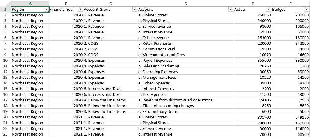
Now, you need to ensure your data is in a tabular format. This means your data respects the following conditions:

Every record is housed in one row.
Each Column contains a type of data.
There are no blank rows or columns.
There are no subtotals or totals in the data.

In this example, we have added the Account Group column to represent different sections of the report and have named the table containing the data tblIncome.

Pivot

Insert the Pivot Table

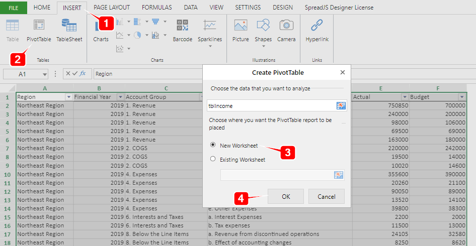
If you are using our Designer Component, insert the PivotTable following these steps:

Select tblIncome table
On the Insert tab, click PivotTable
Choose "New Worksheet"
Ok, at the end

JavaScript Income Statement

Or you can add it using the below code if you are using javascript:

let pivotTable = sheet.pivotTables.add("myPivotTable", "tblIncome", 1, 1);

Build the Pivot Table

To exactly build the PivotTable, we will be using the PivotTable Panel. If you are using Designer, the panel will be shown at the right of the sheet every time you click on the PivotTable.

You can also add it to your javascript instance using the code below:

var pt = spread.getActiveSheet().pivotTables.all()[0]; 

var panel = new GC.Spread.Pivot.PivotPanel('myPivotPanel', pt, document.getElementById("panel")); 

panel.sectionVisibility(GC.Spread.Pivot.PivotPanelSection.fields |GC.Spread.Pivot.PivotPanelSection.area);

Drag and drop the fields on the right areas to build the PivotTable. In our example, the Account Group and Account field to the Rows and add Actual and Budget to the Values.

JavaScript Income Statement

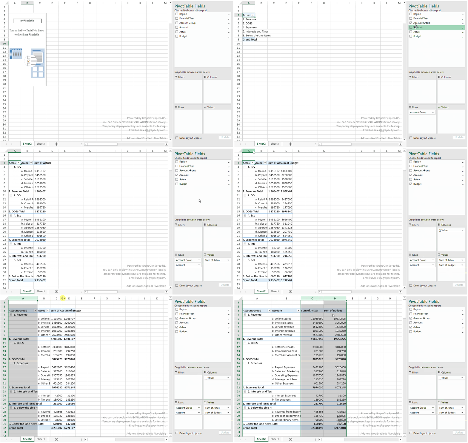
Notice: The PivotTable can work without PivotPanel; we have just added it for ease of use.

Add Calculated Items

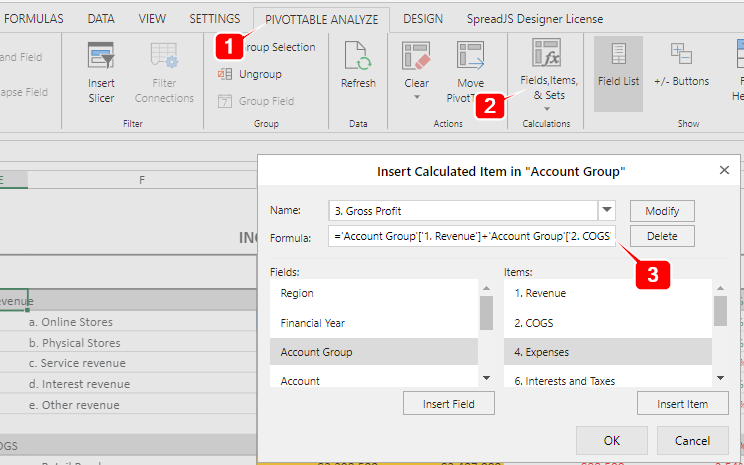
In addition to the existing items in a pivot table field, you can create one or more calculated items using custom formulas.

Click PivotTable Analyze
Fields, Items & Sets → Calculated Item
Set the name 3. Gross Profit and as formula: ='Account Group'['1. Revenue']-'Account Group'['2. COGS']

Add the calculated Item using only the code as follows:

pivotTable.addCalcItem("Account Group", "3. Gross Profit","='Account Group'['1. Revenue']-'Account Group'['2. COGS']");

Add the other Calculated Items following the above steps. The formulas for those are shown in the table below:

Item	Formula
'3. Gross Profit'	='Account Group'['1. Revenue']-'Account Group'['2. COGS']
'5. EBIT'	='Account Group'['3. Gross Profit']-'Account Group'['4. Expenses']
'7. Income from Continuing Operations'	='Account Group'['5. EBIT']-'Account Group'['6. Interests and Taxes']
'9. Net Profit'	='Account Group'['7. Income from Continuing Operations']+'Account Group'['8. Below the Line Items']

This will make your JavaScript Income Statement more readable for the user.

Add Calculated Fields

Income Statements often use the Variance Analysis for performance comparison. A budget variation is positive or favorable when actual revenue returns are higher than budget projections or expenses are lower than budget.

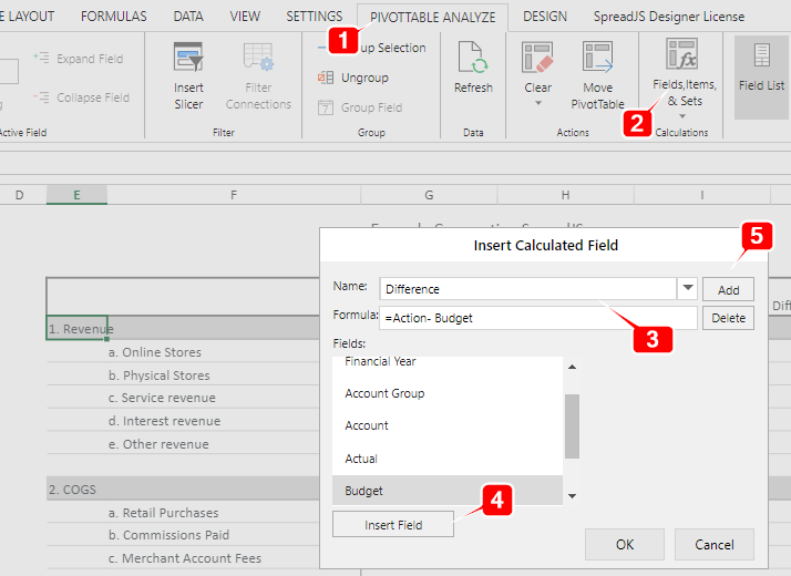
We will use the Calculated Fields feature to add the Difference and Difference % on our PivotTable.

Click PivotTable Analyze.
Fields, Items & Sets → Calculated Field.
Set the name, Difference, of the calculated field.
To add the fields on the formula, select the field and then click Insert Field.
Click the Add button.

Fields

JavaScript code:

pivotTable.addCalcField('diff', '=Actual-Budget'); 
pivotTable.add("diff", "Difference", GC.Spread.Pivot.PivotTableFieldType.valueField); 

pivotTable.addCalcField('diff%', '=Actual/Budget-1'); 
pivotTable.add("diff%", "Difference %", GC.Spread.Pivot.PivotTableFieldType.valueField);

The two fields we have added are Difference and Difference %. The formulas used are as follows:

Field	Formula
Difference	=Actual-Budget
Difference %	=Actual/Budget-1

Add Slicers

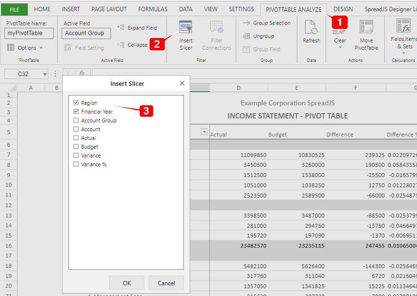
On our SpreadJS v15 release, we added Slicers as a new feature to filter your PivotTable. Use this feature to filter your data by Region and Financial Year.

If you are using Designer Component, do as follows:

Click PivotTable Analyze
Insert Slicer
Select Region and Financial Year

To add slicers in JavaScript, use the code below:

var regionSlicer = sheet.slicers.add("Region", pivotTable.name(), "Region", GC.Spread.Sheets.Slicers.SlicerStyles.dark1(), GC.Spread.Sheets.Slicers.SlicerType.pivotTable); 
var yearSlicer = sheet.slicers.add("Financial Year", pivotTable.name(), "Financial Year", GC.Spread.Sheets.Slicers.SlicerStyles.dark4(), GC.Spread.Sheets.Slicers.SlicerType.pivotTable);

Make Some Appearance Adjustments

For the PivotTable to be more easily read, make some adjustments like:

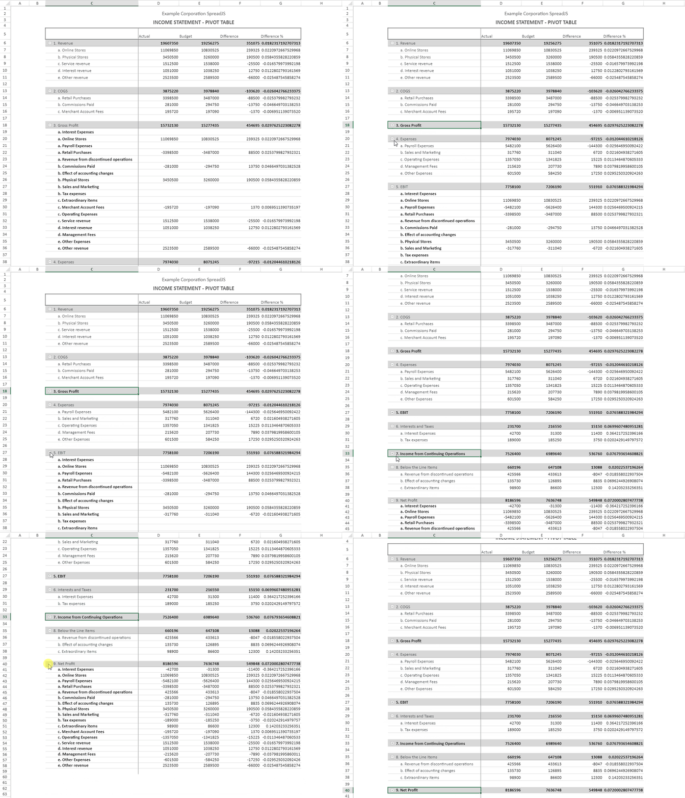
Collapse the Calculated Items

This will hide the accounts summed to show the value of the calculated Item.

JavaScript Income Statement

Show SubTotals at the Top of the Group *

Go to the Design tab.
Click Subtotals
Select "Show all SubTotals at the Top of the Group"

Subtotal

Insert Blank Line after Each Item *

Go to the Design tab.
Click Blank Rows
Select "Insert Blank Line after Each Item"

Blank

Hide Buttons and Field Headers *

Go to the PivotTable Analyze tab.
Click Buttons and Field Headers

Change the Pivot Layout *

Go to the Design tab.
Click Report Layout
Select "Show in Outline Form"

Layout

The modifications mentioned above can be easily changed via code. SpreadJS provides many different options to customize the appearance and functionality of the PivotTables according to the needs of your application. You can change the PivotTables options and the layout as below:

let option = pivotTable.options;
option = {
        allowMultipleFiltersPerField: true,
        insertBlankLineAfterEachItem: true, // Insert Blank Line after Each Item *
        grandTotalPosition: GC.Spread.Pivot.GrandTotalPosition.row,
        subtotalsPosition: GC.Spread.Pivot.SubTotalsPosition.top, // Show SubTotals at the Top of the Group *
        displayFieldsInPageFilterArea: GC.Spread.Pivot.DisplayFields.downThenOver,
        reportFilterFieldsPerColumn: 1,
        bandRows:true,
        bandColumns: true,
        showRowHeader: true,
        showColumnHeader: true,
        showDrill: true, // Collapse Buttons *
        showMissing: true,
        showToolTip: true,
        missingCaption: 'something',
        fillDownLabels: false,
        repeatAllItemLabels: false,
        rowLabelIndent: 4,
        mergeItem: false,
        showHeaders: true // Collapse Field Headers *
    };
pivotTable.layoutType(1); // Change the Pivot Layout to Outline Form *

Conditional and Custom Formatting

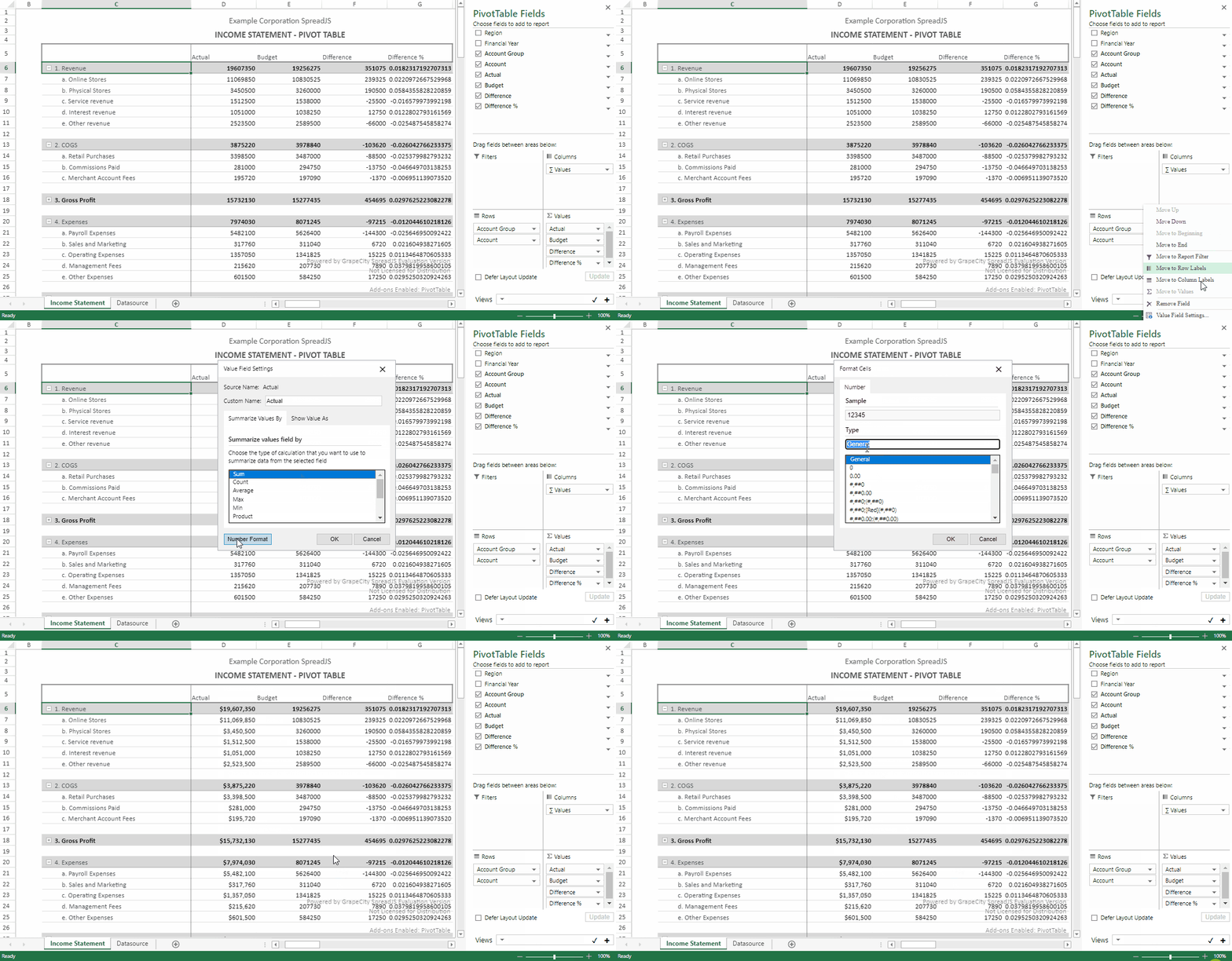
Next, we are going to format the PivotTable fields. You can set the format using the pivot panel as below:

Go to Values - > Value Field Settings
Click Number Format
Set Format. In our case: $#,##0
Confirm.

Format

If you want to do that by code, see below:

//identify the area
var areaActual= {
            dataOnly: true,
            references: [
                {
                    fieldName: "Actual",
                    items: [fieldName]
                }
            ]
        };
 
var style = new GC.Spread.Sheets.Style();
style.formatter = "$#,##0";
//set style to the area
pivotTable.setStyle(areaActual, style);

We can use the same logic for the other fields. Use the corresponding formats in the table below:

Field	Format
Budget	$#,##0
Difference	[Green]$#,##0;[Red]\-$#,##0
Difference %	[Green]0.00%;[Red]\-0.00%

We recommend using Conditional Formatting to make it quicker for the viewer to see the biggest accounts. PivotTables offers the ability to set conditional rules to the specified dimensions. No matter how the PivotTable layout changes, the conditional rules only follow the specified dimensions.

If you are using Designer, follow the below steps to add conditional formatting rules:

Select the cells: G7:H11
Home → Conditional Formating → New Rule.
Choose "Format all cells based on their values".
Format style: 2-Color Scale (blue for the highest value, white for the lowest).

Conditional

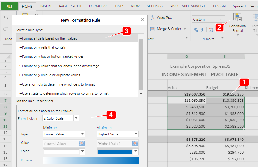
Repeat the same for other Account Groups, considering using Yellow for the Expenses and Blue for the Incomes.

Final Report

Below, you have a screenshot of what your Income Statement Report would look like at the end:

Final Report

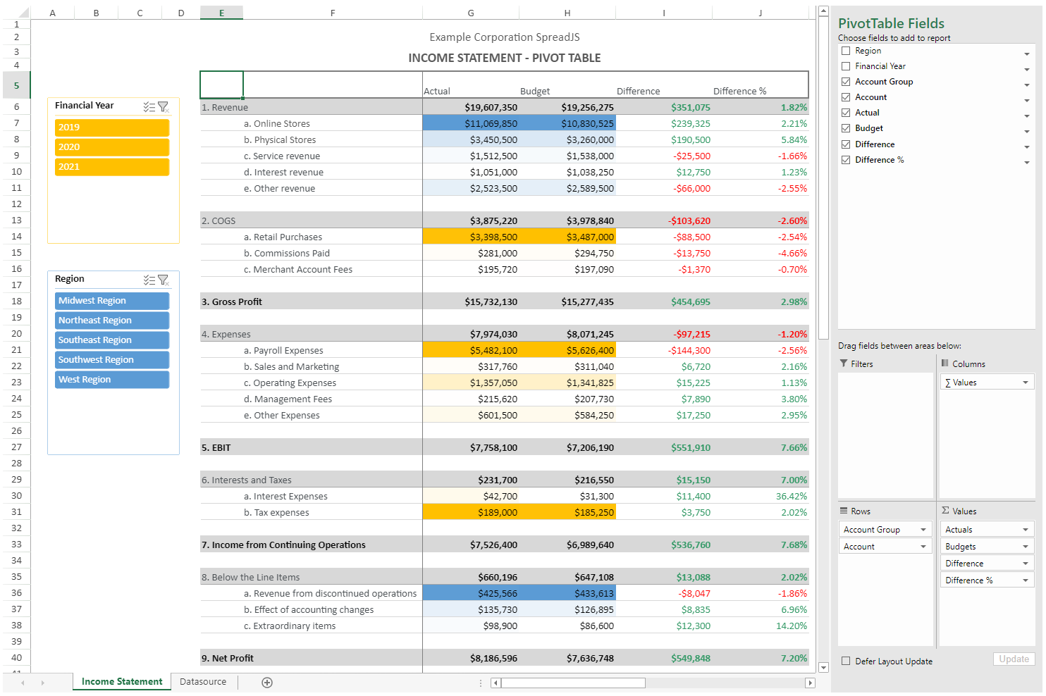
You can then load this into your application by first exporting as a JavaScript file using File>Export>SpreadJS JSON>Export JavaScript Files:

Export JavaScript Files

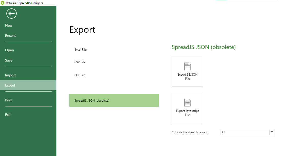
Once the file is saved within your project, you can add a script reference to the head section of the HTML:

<script src="data.js" type="text/javascript"></script>

This is how you can use our JavaScript component for generating the needed financial reports to assess your retail business performance and set the stage for discovering insights that can influence decision-making and drive change with a JavaScript income statement.

Discover more about the opportunities SpreadJS offers by getting the free trial.

If you have any questions or insights you would like to share, please post a comment below. Thanks!