Drop-down Lists and Dynamic Array Formulas in Spread.NET 12 Windows Forms

Using the new Dynamic Array Formulas available in Spread.NET 12 Windows Forms, you can easily create dependent drop-down lists and use them to generate a filtered report. This blog describes how to create such a report using three simple formulas and data validation.

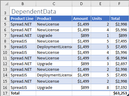
This example uses the following table DependentData for sample data:

A simple formula using the UNIQUE function can return the list of unique values in the Product Line column to create contents for the first drop-down list:

=UNIQUE(DependentData[Product Line])

Another simple formula, also using the UNIQUE function, can return the list of unique values in the Product column to create the contents for the second drop-down list:

=UNIQUE(FILTER(DependentData[Product],DependentData[Product Line]=H5,"None Found"))

Note that the above formula uses the value in the cell H5 to filter the contents of the Product column, together with the UNIQUE function to ensure each value shows only once.

These formulas must be set in cell ranges to generate the list contents, as these dynamic array formulas are not supported directly in the data validation condition formula.

You can specify a dynamic array cell reference for the data validation list ranges:

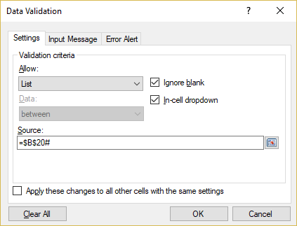
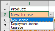
Figure 6-7 - Data Validation list settings for the cell J5.

Now the drop-down lists can generate a nice report of the DependentData table using the FILTER function and cells H5 and J5:

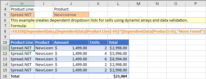
=FILTER(DependentData,(DependentData[Product Line]=H5)*(DependentData[Product]=J5),"None Found")

The Total in row 16 was added manually, and the formatting in the cells H11:L15 is added using conditional formatting to appear like a table:

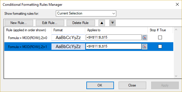
The formulas for the conditional formatting use the ROW function to apply a formula rule that creates the alternating row styles, and the styles are simply alternating between using a fill and top and bottom borders using the same color.

Searchable Drop-down List

You can also create a searchable drop-down list using dynamic array formulas in a cell range. A searchable drop-down list displays only the items which match the text typed into the cell.

This example uses the following table SearchableData for sample data:

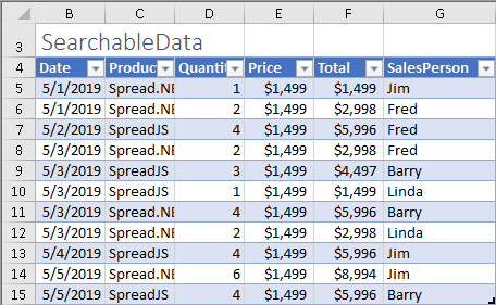
The formula to generate the list of items for the data validation drop-down is more complex in this case, using UNIQUE, FILTER, ISNUMBER, and SEARCH:

=UNIQUE(FILTER(G5:G15,ISNUMBER(SEARCH(I8,G5:G15)),G5:G15))

The formula uses the SEARCH function with the cell range G5:G15 for the second argument, which is normally a scalar value. This causes the calculation engine to "lift" the calculation and calculate SEARCH for each value in G5:G15, then return the result in a dynamic array. That resulting array is then passed to ISNUMBER, which returns TRUE or FALSE for each value and returns the result in another dynamic array. That result is then passed to FILTER, which returns the filtered list of names, and finally UNIQUE ensures that each name appears only once in the list.

The data validation for the cell I8 references the dynamic array result in H5#:

Figure 12 - Data validation list settings for the cell I8

It is also important to uncheck the box for "Show error alert after invalid data is entered" in the "Error Alert" tab:

Figure 13 Data Validation error alert settings for the cell I8

Now the drop-down list will show different content when a search value is typed in the cell then the list is shown:

Figures 14-15 Data validation lists showing different values