


- Spread for WPF Overview
- About the Product
- Getting Started
- Quick Start
- Designer
- Features
- Assembly Reference
3-D Rotation
Spread for WPF allows users to enhance data visualization with the rotation feature of 3D charts. You can use the following properties of the IChart interface to set the 3-D rotation and perspective effects of a 3D chart:
Perspective:The degree of perspective effect, influencing how depth is perceived in the 3D chart.
Rotation:The rotation angle of the chart around its vertical axis (Y-axis).
Elevation:Determines the angle at which the chart is viewed from the horizontal plane.
RightAngleAxes:Determines whether the axes are displayed at right angles. This property applies only to 3D line, column, and bar charts.
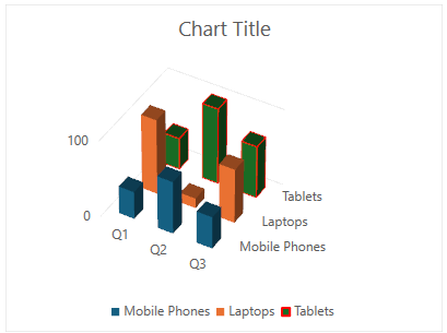
Refer to the following example code to change the rotation and perspective effects of a 3D chart.
// Add data.
object[,] dataArray = {
     {"", "Q1", "Q2", "Q3"},
     {"Mobile Phones", 36, 69, 42},
     {"Laptops", 98, 13, 71},
     {"Tablets", 41, 99, 68}
};
for (int i = 0; i < dataArray.GetLength(0); i++)
{
    for (int j = 0; j < dataArray.GetLength(1); j++)
    {
        spreadSheet1.Workbook.ActiveSheet.Cells[i, j].Value = dataArray[i, j];
    }
}
spreadSheet1.Workbook.ActiveSheet.Cells["A1:D4"].Select();
// Add Column3D chart.
spreadSheet1.Workbook.ActiveSheet.Shapes.AddChart(GrapeCity.Spreadsheet.Charts.ChartType.Column3D, 100, 150, 400, 300, true);
// Configure axis.
var valueAxis = spreadSheet1.Workbook.ActiveSheet.ChartObjects[0].Chart.Axes[AxisType.Value];
valueAxis.MaximumScale = 100;
valueAxis.MajorUnit = 100;
valueAxis.MinorUnit = 20;
// Configure 3-D rotation properties.
spreadSheet1.Workbook.ActiveSheet.ChartObjects[0].Chart.Perspective = 10;
spreadSheet1.Workbook.ActiveSheet.ChartObjects[0].Chart.RightAngleAxes = false;
spreadSheet1.Workbook.ActiveSheet.ChartObjects[0].Chart.Rotation = 30;
spreadSheet1.Workbook.ActiveSheet.ChartObjects[0].Chart.Elevation = 40;
// Configure the line style of the series "Tablet".
spreadSheet1.Workbook.ActiveSheet.ChartObjects[0].Chart.Series[2].Format.Line.BackColor.Color = GrapeCity.Core.SchemeColor.CreateArgbColor(255, 0, 0);
spreadSheet1.Workbook.ActiveSheet.ChartObjects[0].Chart.Series[2].Format.Line.Weight = 2;
' Add data.
Dim dataArray(,) As Object = {
{"", "Q1", "Q2", "Q3"},
{"Mobile Phones", 36, 69, 42},
{"Laptops", 98, 13, 71},
{"Tablets", 41, 99, 68}
}
For i As Integer = 0 To dataArray.GetLength(0) - 1
For j As Integer = 0 To dataArray.GetLength(1) - 1
spreadSheet1.Workbook.ActiveSheet.Cells(i, j).Value = dataArray(i, j)
Next
Next
spreadSheet1.Workbook.ActiveSheet.Cells("A1:D4").Select()
' Add Column3D chart.
spreadSheet1.Workbook.ActiveSheet.Shapes.AddChart(GrapeCity.Spreadsheet.Charts.ChartType.Column3D, 100, 150, 400, 300, True)
' Configure axis.
Dim valueAxis = spreadSheet1.Workbook.ActiveSheet.ChartObjects(0).Chart.Axes(GrapeCity.Spreadsheet.Charts.AxisType.Value)
valueAxis.MaximumScale = 100
valueAxis.MajorUnit = 100
valueAxis.MinorUnit = 20
' Configure 3-D rotation properties.
With spreadSheet1.Workbook.ActiveSheet.ChartObjects(0).Chart
.Perspective = 10
.RightAngleAxes = False
.Rotation = 30
.Elevation = 40
End With
' Configure the line style of the series "Tablet".
spreadSheet1.Workbook.ActiveSheet.ChartObjects(0).Chart.Series(2).Format.Line.BackColor.Color = GrapeCity.Core.SchemeColor.CreateArgbColor(255, 0, 0)
spreadSheet1.Workbook.ActiveSheet.ChartObjects(0).Chart.Series(2).Format.Line.Weight = 2