
-
Spread Windows Forms Product Documentation
- Getting Started
-
Developer's Guide
- Understanding the Product
- Working with the Component
- Spreadsheet Objects
- Ribbon Control
- Sheets
- Rows and Columns
- Headers
- Cells
- Cell Types
- Data Binding
- Customizing the Sheet Appearance
- Customizing Interaction in Cells
- Tables
- Pivot Table
- Understanding the Underlying Models
- Customizing Row or Column Interaction
- Formulas in Cells
-
Sparklines
- Add Sparklines Using Methods
-
Add Sparklines using Formulas
- Column, Line, and Winloss Sparkline
- Area Sparkline
- BoxPlot Sparkline
- Bullet Sparkline
- Cascade Sparkline
- Gauge KPI Sparkline
- Hbar and Vbar Sparkline
- Histogram Sparkline
- Image Sparkline
- Month and Year Sparkline
- Pareto Sparkline
- Pie Sparkline
- Scatter Sparkline
- Spread Sparkline
- Stacked Sparkline
- Vari Sparkline
- Keyboard Interaction
- Events from User Actions
- File Operations
- Storing Excel Summary and View
- Printing
- Chart Control
- Enhanced Chart
- Customizing Drawing
- Touch Support with the Component
- Spread Designer Guide
- Assembly Reference
- Import and Export Reference
- Version Comparison Reference
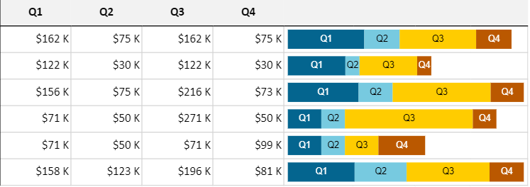
Stacked Sparkline
A stacked sparkline is used to show a sliced breakdown of a value in different categories. It is useful for comparing values across categories as shown in the image below.
The stacked sparkline formula has the following syntax:
=STACKEDSPARKLINE(points, [colorRange, labelRange, maximum, targetRed, targetGreen, targetBlue, tragetYellow, color, highlightPosition, vertical, textOrientation, textSize, minimum])
The formula options are described below:
Option | Description |
|---|---|
points | A reference that represents a range of cells that contains the values, such as "A1:A4". |
colorRange Optional | A reference that represents a range of cells that contains all colors, such as "B1:B4". The default value is generated by color. |
labelRange Optional | A reference that represents a cell range that contains all labels, such as "C1:C4". The default value is empty. |
maximum Optional | A number that represents the maximum value of the sparkline. The default value is the summary of all positive values. |
targetRed Optional | A number that represents the location of the red line. This setting is optional. The default value is empty. |
targetGreen Optional | A number that represents the location of the green line. The default value is empty. |
targetBlue Optional | A number that represents the location of the blue line. The default value is empty. |
targetYellow Optional | A number that represents the location of the yellow line. The default value is empty. |
color Optional | A string that represents the color if colorRange is omitted. The default value is "#646464". |
highlightPosition Optional | A number that represents the index of the highlight area. The default value is empty. |
vertical Optional | A boolean that represents whether to display the sparkline vertically. The default value is false. |
textOrientation Optional | A number that represents the label text orientation. The default value is 0 (horizontal). The vertical setting is 1. |
textSize Optional | A number that represents the size of the label text in pixels. The default value is 10. |
minimum Optional | A number that represents the minimum axis value. The default value is 0. |
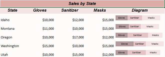
Usage Scenario
Consider a scenario where a company wants to display the sales of products in different US states. Stacked sparklines can show each US state divided into the shares of the company products.
// Get sheet
var worksheet = fpSpread1_Sheet1.AsWorksheet();

// Add data for sparkline
worksheet.SetValue(1, 0, "State");
worksheet.SetValue(1, 1, "Gloves");
worksheet.SetValue(1, 2, "Sanitizer");
worksheet.SetValue(1, 3, "Masks");
worksheet.SetValue(1, 4, "Diagram");
worksheet.SetValue(2, 0, "Idaho");
worksheet.SetValue(2, 1, 10000);
worksheet.SetValue(2, 2, 12000);
worksheet.SetValue(2, 3, 15000);
worksheet.SetValue(3, 0, "Montana");
worksheet.SetValue(3, 1, 11000);
worksheet.SetValue(3, 2, 10000);
worksheet.SetValue(3, 3, 15000);
worksheet.SetValue(4, 0, "Oregon");
worksheet.SetValue(4, 1, 10000);
worksheet.SetValue(4, 2, 17000);
worksheet.SetValue(4, 3, 12000);
worksheet.SetValue(5, 0, "Washington");
worksheet.SetValue(5, 1, 15000);
worksheet.SetValue(5, 2, 10000);
worksheet.SetValue(5, 3, 15000);
worksheet.SetValue(6, 0, "Utah");
worksheet.SetValue(6, 1, 10000);
worksheet.SetValue(6, 2, 15000);
worksheet.SetValue(6, 3, 12000);
worksheet.SetValue(7, 1, "#B39A9A");
worksheet.SetValue(7, 2, "#E3C3C3");
worksheet.SetValue(7, 3, "#F5E4E4");

// Set number format for columns
worksheet.Columns["B:D"].NumberFormat = "$#,##0";

// Set StackedSparkline formula
worksheet.Cells[2, 4].Formula = "STACKEDSPARKLINE(B3:D3,B8:D8,B2:D2,40000)";
worksheet.Cells[3, 4].Formula = "STACKEDSPARKLINE(B4:D4,B8:D8,B2:D2,40000)";
worksheet.Cells[4, 4].Formula = "STACKEDSPARKLINE(B5:D5,B8:D8,B2:D2,40000)";
worksheet.Cells[5, 4].Formula = "STACKEDSPARKLINE(B6:D6,B8:D8,B2:D2,40000)";
worksheet.Cells[6, 4].Formula = "STACKEDSPARKLINE(B7:D7,B8:D8,B2:D2,40000)";

// Set backcolor for cells
worksheet.Cells["A1"].Interior.Color = GrapeCity.Spreadsheet.Color.FromArgb(unchecked((int)0xFFDEACA7));
worksheet.Cells["A2:E2"].Interior.Color = GrapeCity.Spreadsheet.Color.FromArgb(unchecked((int)0xFFF5E4E4));
worksheet.Cells["A3:E7"].Interior.Color = GrapeCity.Spreadsheet.Color.FromArgb(unchecked((int)0xFFfdfafa));
'Get sheet
Dim worksheet = FpSpread1_Sheet1.AsWorksheet()
'Add data for sparkline
worksheet.SetValue(1, 0, "State")
worksheet.SetValue(1, 1, "Gloves")
worksheet.SetValue(1, 2, "Sanitizer")
worksheet.SetValue(1, 3, "Masks")
worksheet.SetValue(1, 4, "Diagram")
worksheet.SetValue(2, 0, "Idaho")
worksheet.SetValue(2, 1, 10000)
worksheet.SetValue(2, 2, 12000)
worksheet.SetValue(2, 3, 15000)
worksheet.SetValue(3, 0, "Montana")
worksheet.SetValue(3, 1, 11000)
worksheet.SetValue(3, 2, 10000)
worksheet.SetValue(3, 3, 15000)
worksheet.SetValue(4, 0, "Oregon")
worksheet.SetValue(4, 1, 10000)
worksheet.SetValue(4, 2, 17000)
worksheet.SetValue(4, 3, 12000)
worksheet.SetValue(5, 0, "Washington")
worksheet.SetValue(5, 1, 15000)
worksheet.SetValue(5, 2, 10000)
worksheet.SetValue(5, 3, 15000)
worksheet.SetValue(6, 0, "Utah")
worksheet.SetValue(6, 1, 10000)
worksheet.SetValue(6, 2, 15000)
worksheet.SetValue(6, 3, 12000)
worksheet.SetValue(7, 1, "#B39A9A")
worksheet.SetValue(7, 2, "#E3C3C3")
worksheet.SetValue(7, 3, "#F5E4E4")
'Set number format for columns
worksheet.Columns("B:D").NumberFormat = "$#,##0"
'Set StackedSparkline formula
worksheet.Cells(2, 4).Formula = "STACKEDSPARKLINE(B3:D3,B8:D8,B2:D2,40000)"
worksheet.Cells(3, 4).Formula = "STACKEDSPARKLINE(B4:D4,B8:D8,B2:D2,40000)"
worksheet.Cells(4, 4).Formula = "STACKEDSPARKLINE(B5:D5,B8:D8,B2:D2,40000)"
worksheet.Cells(5, 4).Formula = "STACKEDSPARKLINE(B6:D6,B8:D8,B2:D2,40000)"
worksheet.Cells(6, 4).Formula = "STACKEDSPARKLINE(B7:D7,B8:D8,B2:D2,40000)"
'Set back color for cells
worksheet.Cells("A1").Interior.Color = GrapeCity.Spreadsheet.Color.FromArgb(&HFFDEACA7)
worksheet.Cells("A2:E2").Interior.Color = GrapeCity.Spreadsheet.Color.FromArgb(&HFFF5E4E4)
worksheet.Cells("A3:E7").Interior.Color = GrapeCity.Spreadsheet.Color.FromArgb(&HFFFDFAFA)Using the Spread Designer
Type data in a cell or a column or row of cells in the designer.
Select a cell for the sparkline.
Select the Insert menu.
Select a sparkline type.
Set the Data Range in the Create Sparklines dialog (such as =Sheet1!$E$1:$E$3).
Alternatively, set the range by selecting the cells in the range using the pointer.
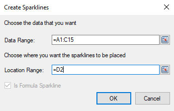
You can also set additional sparkline settings in the dialog if available.
Select OK.
Select Apply and Exit from the File menu to save your changes and close the designer.