Spread Windows Forms Product Documentation

Pie Sparkline

Pie sparkline is a circular statistical diagram, which is divided into slices to illustrate numerical proportion. This sparkline makes it easier to see the percentages of data points compared to the entire set of data.

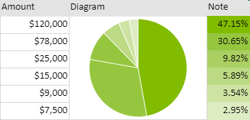
Spread WinForms PIESPARKLINE formula converts six amount values into a pie diagram with corresponding percentage cells and colored sectors.

The pie sparkline formula has the following syntax:

=PIESPARKLINE(percentage, [color1, color2, ...])

The formula options are described below where only 'percentage' is the required argument:

Option	Description
percentage	A value that represents the range of data sources.
color1, color2, ... Optional	Strings that represent the sequence of colors for the pie slices.

Usage Scenario

Consider a scenario where a company analyzes its energy consumption in a month. It wants to display the key areas where it can improve on energy conservation. A pie sparkline can showcase the proportions of different consumption factors in the office campus.

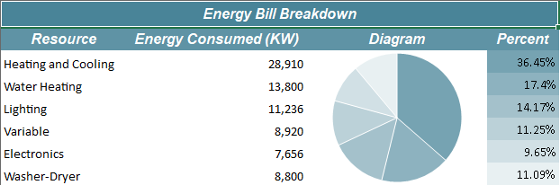
Spread WinForms PIESPARKLINE formula visualizes office energy consumption by resource as a pie diagram with percentage values.

// Get sheet
var worksheet = fpSpread1_Sheet1.AsWorksheet();
            
// Set data for sparkline
worksheet.SetValue(1, 0, new object[,]
{
    { "Resource", "Energy Consumed (KW)", "Diagram", "Percent" },
    { "Heating and Cooling", 28910, null, null },
    { "Water Heating", 13800, null, null },
    { "Lighting", 11236, null, null },
    { "Variable", 8920, null, null },
    { "Electronics", 7656, null, null },
    { "Washer-Dryer", 8800, null, null }
});

// Merge cells of column C
worksheet.Cells["C3:C8"].Merge();
// Apply formula for PieSparkline
worksheet.Cells["C3"].Formula = "PIESPARKLINE(B3:B8,\"#76a3b2\",\"#8db2bf\",\"#a4c1cb\",\"#bbd1d8\",\"#d1e0e5\",\"#e8f0f2\")";

'Get sheet
Dim worksheet = FpSpread1_Sheet1.AsWorksheet() 
       
'Set data for sparkline
worksheet.SetValue(1, 0, New Object(,) {
{"Resource", "Energy Consumed (KW)", "Diagram", "Percent"},
{"Heating and Cooling", 28910, Nothing, Nothing},
{"Water Heating", 13800, Nothing, Nothing},
{"Lighting", 11236, Nothing, Nothing},
{"Variable", 8920, Nothing, Nothing},
{"Electronics", 7656, Nothing, Nothing},
{"Washer-Dryer", 8800, Nothing, Nothing}})

'Merge cells of column C
worksheet.Cells("C3:C8").Merge()

'Apply formula for PieSparkline
worksheet.Cells("C3").Formula = "PIESPARKLINE(B3:B8,""#76a3b2"",""#8db2bf"",""#a4c1cb"",""#bbd1d8"",""#d1e0e5"",""#e8f0f2"")"

Using the Spread Designer

Type data in a cell or a column or row of cells in the designer.
Select a cell for the sparkline.
Select the Insert menu.
Select a sparkline type.
Set the Data Range in the Create Sparklines dialog (such as =Sheet1!$E$1:$E$3).
Alternatively, set the range by selecting the cells in the range using the pointer.

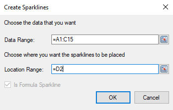
You can also set additional sparkline settings in the dialog if available.
Select OK.
Select Apply and Exit from the File menu to save your changes and close the designer.