
-
Spread Windows Forms Product Documentation
- Getting Started
-
Developer's Guide
- Understanding the Product
- Working with the Component
- Spreadsheet Objects
- Ribbon Control
- Sheets
- Rows and Columns
- Headers
- Cells
- Cell Types
- Data Binding
- Customizing the Sheet Appearance
- Customizing Interaction in Cells
- Tables
- Pivot Table
- Understanding the Underlying Models
- Customizing Row or Column Interaction
- Formulas in Cells
-
Sparklines
- Add Sparklines Using Methods
-
Add Sparklines using Formulas
- Column, Line, and Winloss Sparkline
- Area Sparkline
- BoxPlot Sparkline
- Bullet Sparkline
- Cascade Sparkline
- Gauge KPI Sparkline
- Hbar and Vbar Sparkline
- Histogram Sparkline
- Image Sparkline
- Month and Year Sparkline
- Pareto Sparkline
- Pie Sparkline
- Scatter Sparkline
- Spread Sparkline
- Stacked Sparkline
- Vari Sparkline
- Keyboard Interaction
- Events from User Actions
- File Operations
- Storing Excel Summary and View
- Printing
- Chart Control
- Enhanced Chart
- Customizing Drawing
- Touch Support with the Component
- Spread Designer Guide
- Assembly Reference
- Import and Export Reference
- Version Comparison Reference
Area Sparkline
Area sparklines are presented as a line sparkline graph in which the area between the series and the X axis is filled with color. You can create an area sparkline by using the AREASPARKLINE formula.
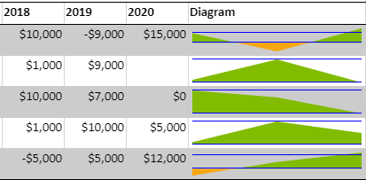
The area sparkline formula has the following syntax:
=AREASPARKLINE(points, [min, max, line1, line2, colorPositive, colorNegative, lineColor])
The formula options are described below:
| Option | Description |
|---|---|
| points | A cell range. Invalid values are treated as 0. |
| min Optional | A number that represents the minimum value of the sparkline. |
| max Optional | A number that represents the maximum value of the sparkline. |
| line1 Optional | A number that represents a horizontal line's vertical position. |
| line2 Optional | A number that represents a second horizontal line's vertical position. |
| colorPositive Optional | A string that represents the area color of positive values. |
| colorNegative Optional | A string that represents the area color of negative values. |
| lineColor Optional | A string that represents the color of the line. |
type=note
Note: In case value of line is smaller than the actual minimum value, the line will not be painted.
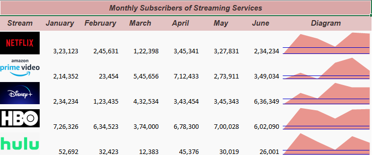
Usage Scenario
Consider a scenario where an entertainment-focused website displays the number of monthly subscribers gained by US-based streaming services. An area sparkline can show the fluctuation throughout the first six months of the year and compare the viewership obtained by those services.
// Get sheet
var worksheet = fpSpread1_Sheet1.AsWorksheet();

// Set data
fpSpread1_Sheet1.AsWorksheet().SetValue(1, 0, new object[,]
{
    {"Stream","January","February","March","April","May","June", "Diagram"},
    { "Netflix",323123,245631,122398,345341,327831,234234, null},
    { "Prime Video",214352,23454,545656,712433,273911,349034, null},
    { "Disney Hotstar",234234,123435,432534,343454,345343,636349, null},
    { "HBO",726326,634523,374000,678300,700028,602090, null},
    { "Hulu",52692,32423,12383,45376,30019,26001,null}
});

// Set backColor for cells
worksheet.Cells["A1"].Interior.Color = GrapeCity.Spreadsheet.Color.FromArgb(unchecked((int)0xFFD9A7A7));
worksheet.Cells["A2:H2"].Interior.Color = GrapeCity.Spreadsheet.Color.FromArgb(unchecked((int)0xFFE3C3C3));
worksheet.Cells["A3:H7"].Interior.Color = GrapeCity.Spreadsheet.Color.FromArgb(unchecked((int)0xFFF9F9F9));
fpSpread1_Sheet1.Cells["A1"].ForeColor = Color.FromArgb(unchecked((int)0xFF3D3131));
fpSpread1_Sheet1.Cells["A2:H2"].ForeColor = Color.FromArgb(unchecked((int)0xFF3D3131));

// Set AreaSparkline formula
worksheet.Cells["H3:H7"].Formula = "Areasparkline(A3:F3,,,0,100000,\"#E9958E\",\"#f7a711\")";
'Get sheet
Dim worksheet = FpSpread1_Sheet1.AsWorksheet()

'Set data
worksheet.SetValue(1, 0, New Object(,) {
{"Stream", "January", "February", "March", "April", "May", "June", "Diagram"},
{"Netflix", 323123, 245631, 122398, 345341, 327831, 234234, Nothing},
{"Prime Video", 214352, 23454, 545656, 712433, 273911, 349034, Nothing},
{"Disney Hotstar", 234234, 123435, 432534, 343454, 345343, 636349, Nothing},
{"HBO", 726326, 634523, 374000, 678300, 700028, 602090, Nothing},
{"Hulu", 52692, 32423, 12383, 45376, 30019, 26001, Nothing}})

'Set backColor for cells
worksheet.Cells("A1").Interior.Color = GrapeCity.Spreadsheet.Color.FromArgb(&HFFD9A7A7)
worksheet.Cells("A2:H2").Interior.Color = GrapeCity.Spreadsheet.Color.FromArgb(&HFFE3C3C3)
worksheet.Cells("A3:H7").Interior.Color = GrapeCity.Spreadsheet.Color.FromArgb(&HFFF9F9F9)
FpSpread1_Sheet1.Cells("A1").ForeColor = Color.FromArgb(&HFF3D3131)
FpSpread1_Sheet1.Cells("A2:H2").ForeColor = Color.FromArgb(&HFF3D3131)

'Set AreaSparkline formula
worksheet.Cells("H3:H7").Formula = "Areasparkline(A3:F3,,,0,100000,""#E9958E"",""#f7a711"")"
Using the Spread Designer
Type data in a cell or a column or row of cells in the designer.
Select a cell for the sparkline.
Select the Insert menu.
Select a sparkline type.
Set the Data Range in the Create Sparklines dialog (such as =Sheet1!$E$1:$E$3).
Alternatively, set the range by selecting the cells in the range using the pointer.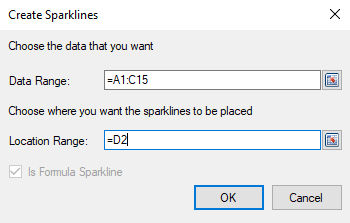
You can also set additional sparkline settings in the dialog if available.
Select OK.
Select Apply and Exit from the File menu to save your changes and close the designer.