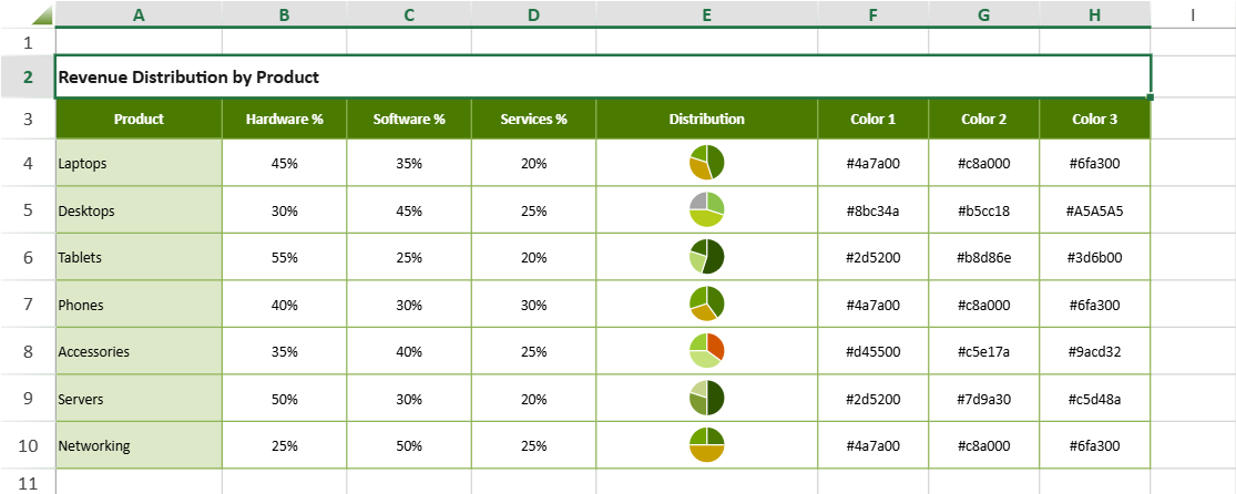
Sparkline Rule

A Sparkline Rule allows you to render cell values as sparklines through conditional formatting.

Instead of inserting sparkline formulas into individual cells, you can apply a Sparkline Rule to a range. The rule automatically generates and renders sparklines for each cell in that range.

It introduces built-in context identifiers that automatically align sparkline configuration with the rule range and the current cell, eliminating hardcoded references.

When to Use a Sparkline Rule

Use a Sparkline Rule when:

• Applying sparklines to a full column, row or range

• When adding Sparklines to a highly correlated data region, such as worksheet table, TableSheet or DataManager, ReportSheet template.

• To avoid altering the original cell data, avoid using formula-based sparkline injection.

• Managing visual rules through conditional formatting priority

How Sparkline Rule Differs from Formula-Based Sparklines

Traditional sparklines are inserted by writing a sparkline function in each cell.

Each formula must explicitly define its data range and, when necessary, the point index.

A Sparkline Rule works differently:

• A single rule is applied to a range.

• Each cell in that range is rendered as a sparkline.

• The rule automatically resolves:

  • The full rule range

  • The current cell value

  • The current cell position within the rule range

This behavior is enabled by two built-in context identifiers

Built-in Context Identifiers

Sparkline conditional formatting rules support two identifiers:

These identifiers may be used:

• As the entire parameter value (for example: value: '@', points: '$CF_RANGE$')

• Inside expressions (for example: IF(@>0,@,0), SUM($CF_RANGE$))

Structured references such as [@Sales] or Table1[@[Column1]:[Column2]] retain their original meaning and are not treated as placeholders.

$CF_RANGE$ — Rule-Level Context

$CF_RANGE$ represents the current range to which the Sparkline Rule is applied.

It always resolves to the rule’s effective conditional formatting range.

• If the rule applies to B1:B5, $CF_RANGE$ resolves to B1:B5.

• If the rule is resized to B1:B10, $CF_RANGE$ automatically resolves to B1:B10.

Instead of hardcoding a data range such as:

dataRange: "A1:A5"

you can write:

dataRange: "$CF_RANGE$"

Example:

sheet.conditionalFormats.addSparklineRule(
    "HISTOGRAMSPARKLINE",
    {
        dataRange: "$CF_RANGE$"
    },
    [new GC.Spread.Sheets.Range(0, 0, 5, 1)]
);

Benefits

• Automatically follows rule range changes

• Eliminates hardcoded references

• Supports expression usage such as SUM($CF_RANGE$)

• Improves rule portability and reuse

@ — Cell-Level Context

@ represents the current cell within the rule range.

Its meaning depends on the parameter in which it is used:

• In index → 0-based index of the current cell within $CF_RANGE$

• In pointIndex → 1-based index of the current cell within $CF_RANGE$

• In other parameters → the current cell value

If @ appears inside a structured reference (for example, [@Sales]), it keeps its structured-reference meaning.

If @ is embedded in an expression and the current cell is blank, it resolves to an empty string literal to ensure the expression remains valid.

Some sparkline types use index (0-based), while others use pointIndex (1-based). Refer to the API reference for type-specific parameter definitions.

Example 1: Using @ for Value and Index

The following example creates a fulfillment dashboard.

• In the On-Time KPI column, @ resolves to the current cell value.

• In the Variance vs Target column, @ resolves to the current row's 0-based index inside the rule range.

var sheet = spread.getActiveSheet();

// Title
sheet.addSpan(0, 0, 1, 6);
sheet.setValue(0, 0, "Weekly Fulfillment Dashboard");

// Header
sheet.setArray(1, 0, [[
    "Warehouse",
    "Target Units",
    "Shipped Units",
    "On-Time Rate",
    "On-Time KPI",
    "Variance vs Target"
]]);

// Data
var data = [
    ["North Hub",   1200, 1260, 1.05, 1.05],  // +5%
    ["East Hub",     950,  910, 0.96, 0.96],  // -4%
    ["South Hub",   1100, 1060, 0.96, 0.96],  // -3.6%
    ["West Hub",     780,  820, 1.05, 1.05],  // +5%
    ["Central Hub", 1350, 1290, 0.96, 0.96]   // -4.4%
];

sheet.setArray(2, 0, data);
sheet.getRange(2, 1, data.length, 2).formatter("#,##0");
sheet.getRange(2, 3, data.length, 2).formatter("0.0%");

// Optional column width for better visuals
sheet.getRange("A:D").width(120);
sheet.getRange("E:F").width(220);
sheet.getRange("3:7").height(42);

// Sparkline Rule
var cfs = sheet.conditionalFormats;

// @ = current cell value in E3:E7.
var gaugeRule = cfs.addSparklineRule(
    "GAUGEKPISPARKLINE",
    {
        targetValue: 1, // targetValue = 1 represents a 100% on-time fulfillment goal.
        currentValue: "@",
        minValue: 0,
        maxValue: 1.2,
        showLabel: false,
        gaugeType: 2,
        colorRange: [
            { start: 0, end: 0.9, color: "#D9534F" },
            { start: 0.9, end: 1, color: "#F0AD4E" },
            { start: 1, end: 1.2, color: "#5CB85C" }
        ]
    },
    [new GC.Spread.Sheets.Range(2, 4, data.length, 1)]
);

// @ = current row index inside F3:F7.
var varianceRule = cfs.addSparklineRule(
    "LOLLIPOPVARISPARKLINE",
    {
        plannedValue: "B3:B7",
        actualValue: "C3:C7",
        index: "@",
        reference: 0,
        mini: -0.15,
        maxi: 0.15,
        tickUnit: 0.05,
        legend: true,
        colorPositive: "#5CB85C",
        colorNegative: "#D9534F",
        lollipopHeaderColor: "#3F4E63"
    },
    [new GC.Spread.Sheets.Range(2, 5, data.length, 1)]
);

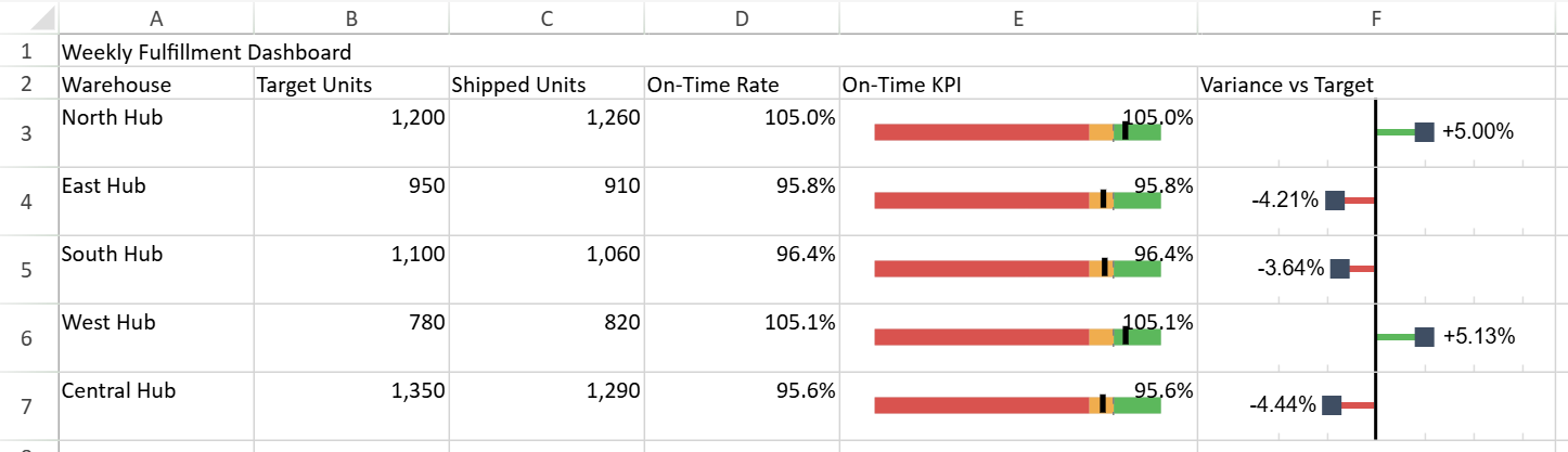
What happens

• In currentValue, @ resolves to each cell's own KPI value in E3:E7.

• In index, @ resolves to 0, 1, 2, 3, and 4 for F3:F7.

• The gauge rule visualizes whether each warehouse meets the 100% service target.

• The lollipop rule compares each row's shipped units against its target without hardcoded row indices.

Example 2: Using $CF_RANGE$ to Eliminate Hardcoded Data Ranges

The following example renders a lollipop variance sparkline for each cell in the Variance column by using the entire rule range as context.

var sheet = spread.getActiveSheet();

// Title
sheet.addSpan(0, 0, 1, 4);
sheet.setValue(0, 0, "Budget Variance Analysis");

// Headers
var headers = ["Department", "Planned ($K)", "Actual ($K)", "Variance"];
sheet.setArray(1, 0, [headers]);

// Data
var data = [
    ["R&D", 850, 760],
    ["Marketing", 420, 500],
    ["Sales", 380, 330],
    ["Support", 260, 305],
    ["Infrastructure", 520, 475]
];

sheet.setArray(2, 0, data);

// Optional column width for better visuals
sheet.getRange("A:D").width(150);

// Sparkline Rule (Advanced Usage)

sheet.conditionalFormats.addSparklineRule(
    "LOLLIPOPVARISPARKLINE",
    {
        // $CF_RANGE$  → D3:D7
        plannedValue: "OFFSET($CF_RANGE$,0,-2)",// Planned column → B
        actualValue: "OFFSET($CF_RANGE$,0,-1)",// Actual column → C
        index: "@",
        reference: 0,
        legend: true,
        colorPositive: "#4CAF50",
        colorNegative: "#E53935"
    },
    [new GC.Spread.Sheets.Range(2, 3, data.length, 1)]// Rule is applied to the Variance column (D3:D7)
);

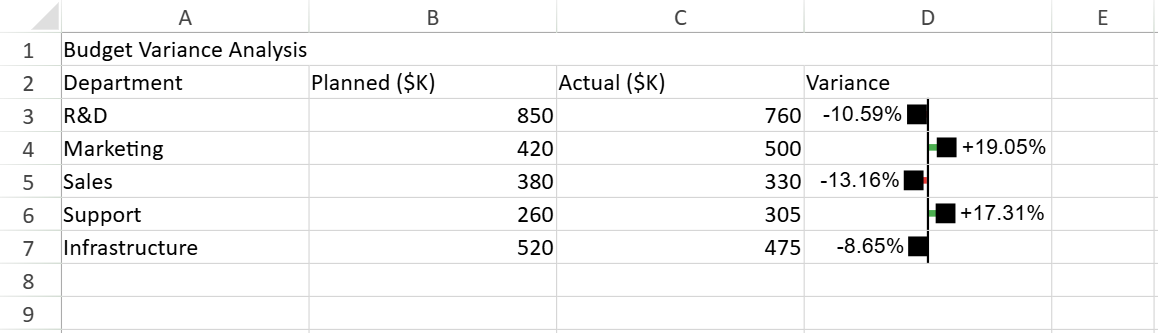
Why this is useful

• The rule always evaluates against the current conditional formatting range.

• Adding or removing rows does not require updating the planned or actual data range.

• The rule remains portable and self-adjusting.

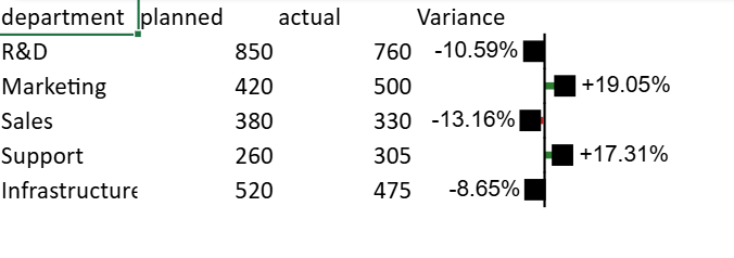
ReportSheet Template Context

When using Sparkline Rules inside a ReportSheet template, the rule is defined on template cells that expand at runtime.

If a sparkline option needs to reference the expanded cell range generated from a template cell, use the R.V(...) formula.

R.V(reference) resolves to the runtime-expanded range corresponding to the specified template cell.

Example:

const spread = new GC.Spread.Sheets.Workbook("ss");
const dataManager = spread.dataManager();

// 1. Data Source
const budgetData = [
    { department: "R&D", planned: 850, actual: 760 },
    { department: "Marketing", planned: 420, actual: 500 },
    { department: "Sales", planned: 380, actual: 330 },
    { department: "Support", planned: 260, actual: 305 },
    { department: "Infrastructure", planned: 520, actual: 475 }
];
dataManager.addTable("Budget", {
    data: budgetData
});

//2. Create ReportSheet
const reportSheet = spread.addSheetTab(
    0,
    "Budget Report",
    GC.Spread.Sheets.SheetType.reportSheet
);
const templateSheet = reportSheet.getTemplate();

const columns = ['department', 'planned', 'actual'];
columns.forEach((columnName, i) => {
    templateSheet.setValue(0, i, `${columnName}`);
    templateSheet.setTemplateCell(1, i, {
        type: 'List',
        binding: `Budget[${columnName}]`,
    });
    templateSheet.setColumnWidth(i, 80)
});
templateSheet.setValue(0, 3, "Variance");
templateSheet.setTemplateCell(1, 3, {
    type: "List"
});
templateSheet.setColumnWidth(3, 150);

//3. Sparkline Rule
templateSheet.conditionalFormats.addSparklineRule(
    "LOLLIPOPVARISPARKLINE",
    {
        plannedValue: "R.V(B2)",
        actualValue: "R.V(C2)",
        index: "@",
        reference: 0,
        legend: true,
        colorPositive: "#2E7D32",
        colorNegative: "#C62828"
    },
    [new GC.Spread.Sheets.Range(1, 3, 1, 1)]
);

// 4. Refresh
reportSheet.refresh();

Explanation

• The Sparkline Rule is defined on template cell D2.

• When the report is refreshed, the template row expands based on the bound data.

• R.V(D2) resolves to the expanded runtime range corresponding to template cell D2.

• index: '@' represents the 0-based position of the current cell within the rule range.

Use R.V(...) in ReportSheet templates when a sparkline option must reference the expanded range generated from a template-bound cell.

Behavior and Policy

• Supported sheet types: Worksheet, TableSheet, ReportSheet

• stopIfTrue is always treated as false for Sparkline Rules

• Relative references are anchored to the origin of the conditional formatting range

• Formula-like option values participate in reference rebasing during copy, move, swap, and sheet rename operations

• Sparkline Rules participate in rule priority ordering

Excel Export

• If Save as View is enabled → exported as images (recommended)

• Otherwise → downgraded to generic Data Bar rules

  • Sparkline-specific visuals are not preserved

  • Only rule priority is retained

Designer Support

When selecting Sparkline as the format style in the Designer:

• The property panel dynamically updates based on the selected sparkline type.

• Certain properties display an Auto option by default:

  • ActualValue defaults to $CF_RANGE$

  • PointIndex defaults to @

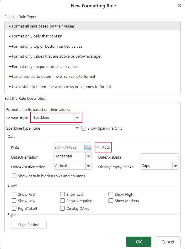
Unchecking Auto allows manual configuration.

See Also

• Sparklines

• Sparkline Functions

• GC.Spread.Sheets.ConditionalFormatting.SparklineRule