Conditional Formatting Dialog
The Conditional Formatting dialog allows you to set up conditional formatting rules. In order to highlight important information in rows or columns of a worksheet, you can create conditional formatting rules for individual cells or a range of cells based on cell values. If the format condition matches with the cell value, the cell is formatted as per the specified rule.
The Conditional Formatting dialog :
Specifies a value or range of values for the rule.
Determines the color of the shading or other formatting options used.
Steps to access the Conditional Formatting dialog:
Select the cell/ cell range you want to format in the worksheet.
Go to the Home tab on the Ribbon.
Click on Conditional Formatting dropdown in the Styles group. A menu with formatting options will appear. Select one of the options to apply conditional formatting to the selected cells. Depending upon the option selected, a dialog box window will appear.
Click OK to apply the conditional formatting to selected cell range.
The following GIF depicts how to apply conditional formatting in the spreadsheet through the designer.
Options in the Conditional Formatting Menu
The Conditional Formatting Menu consists of the following items:
Highlight Cell Rules
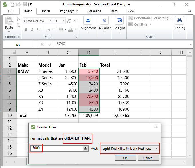
This formatting rule highlight specific cells based on the selected options such as cell value greater than, less than, or equal to a number, and between two numbers. You can also highlight cells that contain specific text, including a specific date.
The image below displays the highlight cell rules applied to cell values in worksheet using designer.
Top/Bottom Rules
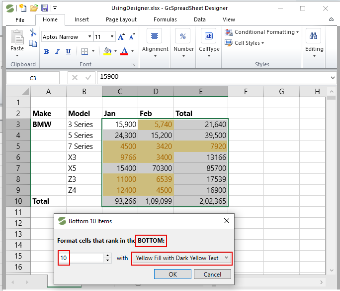
This is a value based formatting rule, used in a worksheet to highlight cell values that meet specific criteria, such as top or bottom 10 percent, above average and below average.
The following image displays the Bottom rule applied on cell values.
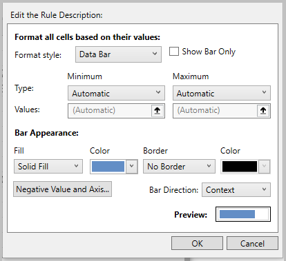
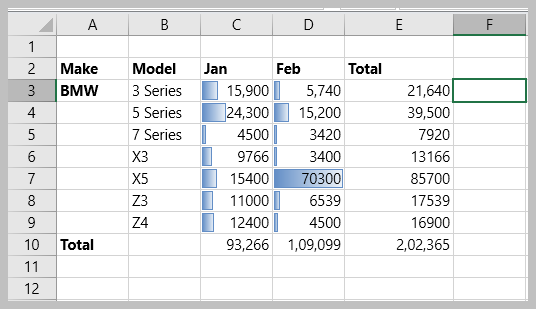
Data Bars
It is a trend-based formatting rule that formats the selected cells with coloured bars. The length of the data bar represents the value in the cell. The longer the bar, the higher the value.
The following image displays the data bar formatting rule applied on selected cell values.
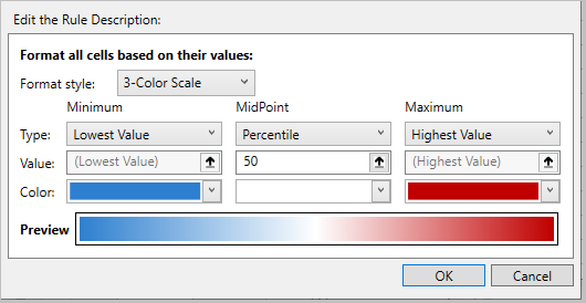
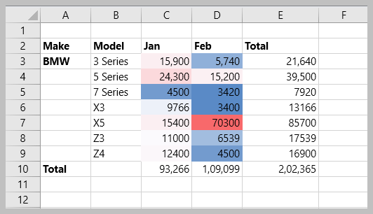
Color Scales
The Color Scale rule helps you visualize data by applying a gradient of colors to a range of cells. This makes it easier to identify high, medium, and low values at a glance. Different shades and colors represent specific values.
The following image displays the conditional formatting applied on cell values using color scales.
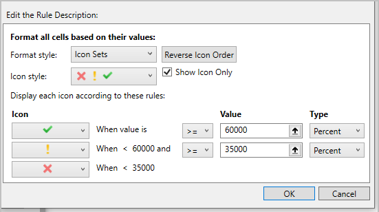
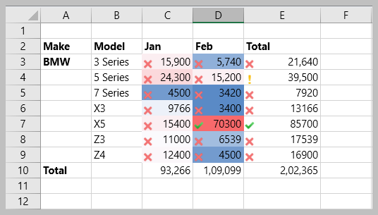
Icon Sets
This trend based formatting option uses different icons to indicate the value of cells relative to each other, making it easy to spot trends and patterns.
The following image displays the formatting using icon sets.
New Rule
This option helps you to select new rule types and edit rule descriptions.
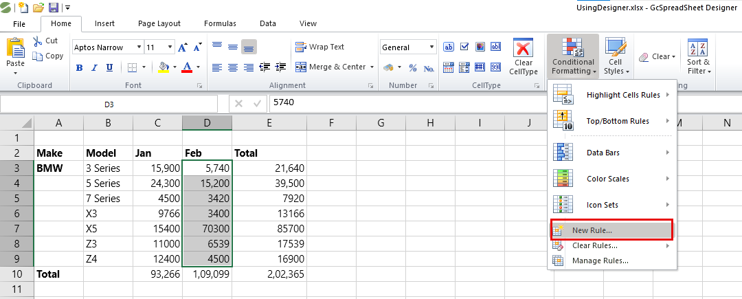
If none of the preset rules meets your needs, you can create a new rule from scratch. To create a new rule, follow these steps:
Select the cells to be formatted and click Conditional Formatting > New Rule… option.
In the New Formatting Rule dialog box that opens, Select the Rule Type: and Edit the Rule Description:
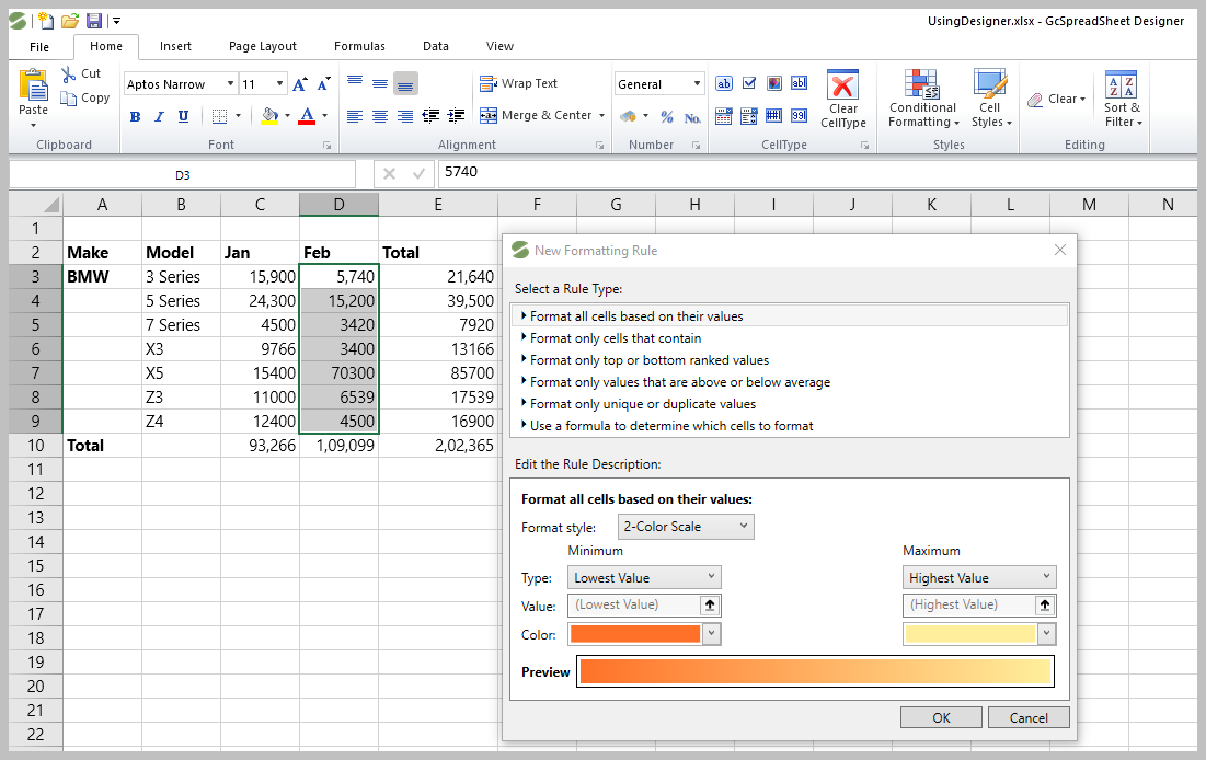
Click OK to close the dialog window and the new conditional formatting rule is created and applied.
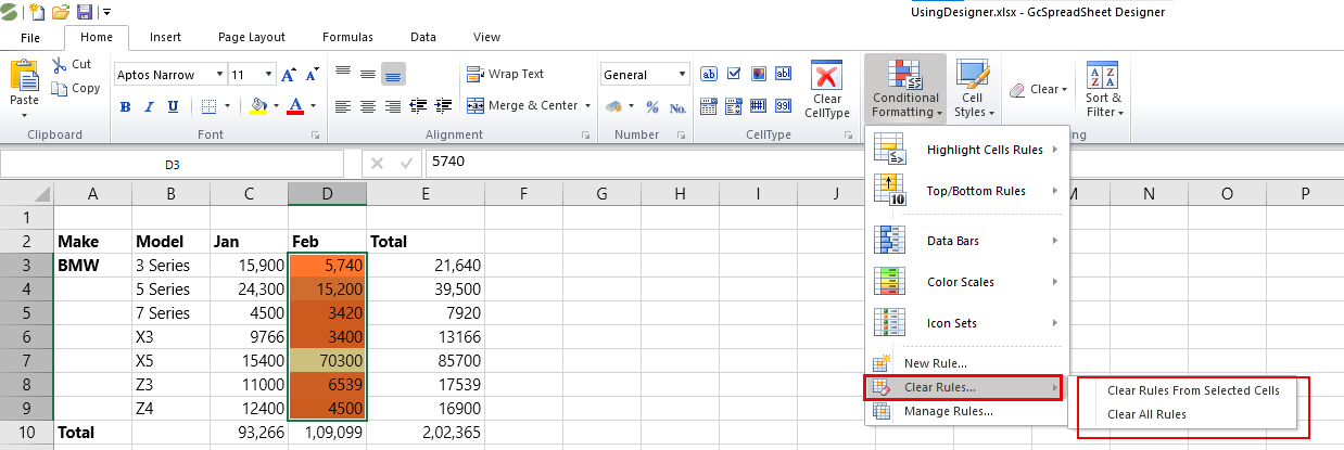
Clear Rules
You can permanently remove a rule from a selected range without affecting other rules for that range. You can delete conditional formatting rules from a worksheet using the Conditional Formatting > Clear Rules… option. You can also clear rules from different elements of your data.
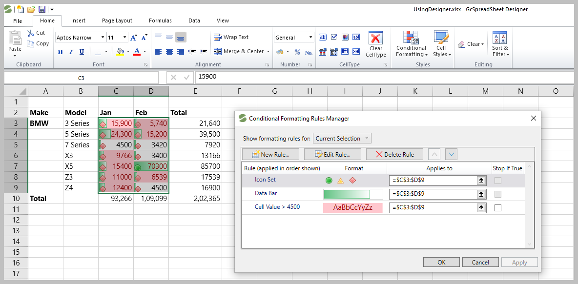
Manage Rules
Conditional formatting rules can be created, edited, deleted and viewed in the Conditional Formatting Rules Manager dialog box. When two or more conditional formatting rules are applied to a range of cells, these rules are evaluated in the order in which they are listed in this dialog box. You can change the order to give some rules precedence over others.
The Stop If True option in conditional formatting prevents the processing of other rules when a condition in the current rule is met. Hence, if two or more rules are set for the same cell and Stop if True option is enabled for the first rule, the subsequent rules are disregarded after the first rule is activated.