Spread Windows Forms Product Documentation

Data Label

Data Labels add specific details to individual data points in a data series. They are used to ensure that users can easily understand and interpret the information plotted in a chart.

You can get or set the data labels, change their position and color, and control whether to show the data labels in the chart using the ApplyDataLabels method of the IChart interface. It returns the members of DataLabelVisibilities enumeration.

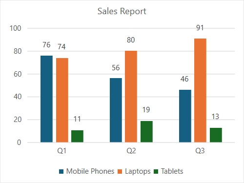
The following example code shows how to configure data labels in a chart.

fpSpread1.Features.EnhancedShapeEngine = true;
fpSpread1.Features.EnhancedChartEngine = true;
fpSpread1.AsWorkbook().ActiveSheet.Cells[0, 1].Value = "Q1";
fpSpread1.AsWorkbook().ActiveSheet.Cells[0, 2].Value = "Q2";
fpSpread1.AsWorkbook().ActiveSheet.Cells[0, 3].Value = "Q3";
fpSpread1.AsWorkbook().ActiveSheet.Cells[1, 0].Value = "Mobile Phones";
fpSpread1.AsWorkbook().ActiveSheet.Cells[2, 0].Value = "Laptops";
fpSpread1.AsWorkbook().ActiveSheet.Cells[3, 0].Value = "Tablets";
Random random = new Random();
for (var r = 1; r <= 3; r++)
{
    for (var c = 1; c <= 3; c++)
    {
        fpSpread1.AsWorkbook().ActiveSheet.Cells[r, c].Value = 0 + random.Next(0, 100);
    }
}
fpSpread1.AsWorkbook().ActiveSheet.Cells["A1:D4"].Select();
fpSpread1.AsWorkbook().ActiveSheet.Shapes.AddChart(GrapeCity.Spreadsheet.Charts.ChartType.ColumnClustered, 100, 150, 400, 300, true);
fpSpread1.AsWorkbook().ActiveSheet.ChartObjects[0].Chart.ChartTitle.Text = "Sales Report";
fpSpread1.AsWorkbook().ActiveSheet.ChartObjects[0].Chart.ApplyDataLabels(DataLabelVisibilities.Value);

fpSpread1.Features.EnhancedShapeEngine = True
fpSpread1.Features.EnhancedChartEngine = True
fpSpread1.AsWorkbook().ActiveSheet.Cells(0, 1).Value = "Q1"
fpSpread1.AsWorkbook().ActiveSheet.Cells(0, 2).Value = "Q2"
fpSpread1.AsWorkbook().ActiveSheet.Cells(0, 3).Value = "Q3"
fpSpread1.AsWorkbook().ActiveSheet.Cells(1, 0).Value = "Mobile Phones"
fpSpread1.AsWorkbook().ActiveSheet.Cells(2, 0).Value = "Laptops"
fpSpread1.AsWorkbook().ActiveSheet.Cells(3, 0).Value = "Tablets"
Dim random As New Random()
For r As Integer = 1 To 3
    For c As Integer = 1 To 3
        fpSpread1.AsWorkbook().ActiveSheet.Cells(r, c).Value = 0 + random.Next(0, 100)
    Next
Next
fpSpread1.AsWorkbook().ActiveSheet.Cells("A1:D4").Select()
fpSpread1.AsWorkbook().ActiveSheet.Shapes.AddChart(GrapeCity.Spreadsheet.Charts.ChartType.ColumnClustered, 100, 150, 400, 300, True)
fpSpread1.AsWorkbook().ActiveSheet.ChartObjects(0).Chart.ChartTitle.Text = "Sales Report"
fpSpread1.AsWorkbook().ActiveSheet.ChartObjects(0).Chart.ApplyDataLabels(DataLabelVisibilities.Value)

Add Shapes to Data Labels

You can use the IDataLabels.Format.AutoShapeType property to customize the shape of data labels for enhanced charts. This property allows you to set the shape of the data labels. It takes the value of GrapeCity.Spreadsheet.Drawing.AutoShapeType enumeration and changes the shape of data labels accordingly.

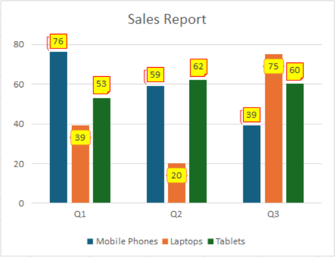
The following example demonstrates how to set different shapes for the data labels of different chart series: Callout3Border, BracePair, and FoldedCorner for series 0, 1, and 2, respectively.

// Enable enhanced shape and chart engines.
fpSpread1.Features.EnhancedShapeEngine = true;
fpSpread1.Features.EnhancedChartEngine = true;
// Set data.
fpSpread1.AsWorkbook().ActiveSheet.Cells[0, 1].Value = "Q1";
fpSpread1.AsWorkbook().ActiveSheet.Cells[0, 2].Value = "Q2";
fpSpread1.AsWorkbook().ActiveSheet.Cells[0, 3].Value = "Q3";
fpSpread1.AsWorkbook().ActiveSheet.Cells[1, 0].Value = "Mobile Phones";
fpSpread1.AsWorkbook().ActiveSheet.Cells[2, 0].Value = "Laptops";
fpSpread1.AsWorkbook().ActiveSheet.Cells[3, 0].Value = "Tablets";
Random random = new Random();
for (var r = 1; r <= 3; r++)
{
    for (var c = 1; c <= 3; c++)
    {
        fpSpread1.AsWorkbook().ActiveSheet.Cells[r, c].Value = 0 + random.Next(0, 100);
    }
}
fpSpread1.AsWorkbook().ActiveSheet.Cells["A1:D4"].Select();
fpSpread1.AsWorkbook().ActiveSheet.Shapes.AddChart(GrapeCity.Spreadsheet.Charts.ChartType.ColumnClustered, 100, 150, 400, 300, true);
fpSpread1.AsWorkbook().ActiveSheet.ChartObjects[0].Chart.ChartTitle.Text = "Sales Report";
// Show data labels and format for series 0.
fpSpread1.AsWorkbook().ActiveSheet.ChartObjects[0].Chart.Series[0].ShowDataLabels = true;
fpSpread1.AsWorkbook().ActiveSheet.ChartObjects[0].Chart.Series[0].DataLabels.Format.Fill.ForeColor.ARGB = System.Drawing.Color.Yellow.ToArgb();
fpSpread1.AsWorkbook().ActiveSheet.ChartObjects[0].Chart.Series[0].DataLabels.Format.Line.ForeColor.ARGB = System.Drawing.Color.Red.ToArgb();
fpSpread1.AsWorkbook().ActiveSheet.ChartObjects[0].Chart.Series[0].DataLabels.Format.AutoShapeType = AutoShapeType.Callout3Border;
// Show data labels and format for series 1.
fpSpread1.AsWorkbook().ActiveSheet.ChartObjects[0].Chart.Series[1].ShowDataLabels = true;
fpSpread1.AsWorkbook().ActiveSheet.ChartObjects[0].Chart.Series[1].DataLabels.Format.Fill.ForeColor.ARGB = System.Drawing.Color.Yellow.ToArgb();
fpSpread1.AsWorkbook().ActiveSheet.ChartObjects[0].Chart.Series[1].DataLabels.Format.Line.ForeColor.ARGB = System.Drawing.Color.Red.ToArgb();
fpSpread1.AsWorkbook().ActiveSheet.ChartObjects[0].Chart.Series[1].DataLabels.Format.AutoShapeType = AutoShapeType.BracePair;
fpSpread1.AsWorkbook().ActiveSheet.ChartObjects[0].Chart.Series[1].DataLabels.Position = DataLabelPosition.InsideEnd;
// Show data labels and format for series 2.
fpSpread1.AsWorkbook().ActiveSheet.ChartObjects[0].Chart.Series[2].ShowDataLabels = true;
fpSpread1.AsWorkbook().ActiveSheet.ChartObjects[0].Chart.Series[2].DataLabels.Format.Fill.ForeColor.ARGB = System.Drawing.Color.Yellow.ToArgb();
fpSpread1.AsWorkbook().ActiveSheet.ChartObjects[0].Chart.Series[2].DataLabels.Format.Line.ForeColor.ARGB = System.Drawing.Color.Red.ToArgb();
fpSpread1.AsWorkbook().ActiveSheet.ChartObjects[0].Chart.Series[2].DataLabels.Format.AutoShapeType = AutoShapeType.FoldedCorner;

' Enable enhanced shape and chart engines.
fpSpread1.Features.EnhancedShapeEngine = True
fpSpread1.Features.EnhancedChartEngine = True
' Set data.
fpSpread1.AsWorkbook().ActiveSheet.Cells(0, 1).Value = "Q1"
fpSpread1.AsWorkbook().ActiveSheet.Cells(0, 2).Value = "Q2"
fpSpread1.AsWorkbook().ActiveSheet.Cells(0, 3).Value = "Q3"
fpSpread1.AsWorkbook().ActiveSheet.Cells(1, 0).Value = "Mobile Phones"
fpSpread1.AsWorkbook().ActiveSheet.Cells(2, 0).Value = "Laptops"
fpSpread1.AsWorkbook().ActiveSheet.Cells(3, 0).Value = "Tablets"
Dim random As New Random()
For r As Integer = 1 To 3
    For c As Integer = 1 To 3
        fpSpread1.AsWorkbook().ActiveSheet.Cells(r, c).Value = random.Next(0, 100)
    Next
Next
fpSpread1.AsWorkbook().ActiveSheet.Cells("A1:D4").Select()
fpSpread1.AsWorkbook().ActiveSheet.Shapes.AddChart(GrapeCity.Spreadsheet.Charts.ChartType.ColumnClustered, 100, 150, 400, 300, True)
fpSpread1.AsWorkbook().ActiveSheet.ChartObjects(0).Chart.ChartTitle.Text = "Sales Report"
' Show data labels and format for series 0.
fpSpread1.AsWorkbook().ActiveSheet.ChartObjects(0).Chart.Series(0).ShowDataLabels = True
fpSpread1.AsWorkbook().ActiveSheet.ChartObjects(0).Chart.Series(0).DataLabels.Format.Fill.ForeColor.ARGB = System.Drawing.Color.Yellow.ToArgb()
fpSpread1.AsWorkbook().ActiveSheet.ChartObjects(0).Chart.Series(0).DataLabels.Format.Line.ForeColor.ARGB = System.Drawing.Color.Red.ToArgb()
fpSpread1.AsWorkbook().ActiveSheet.ChartObjects(0).Chart.Series(0).DataLabels.Format.AutoShapeType = AutoShapeType.Callout3Border
' Show data labels and format for series 1.
fpSpread1.AsWorkbook().ActiveSheet.ChartObjects(0).Chart.Series(1).ShowDataLabels = True
fpSpread1.AsWorkbook().ActiveSheet.ChartObjects(0).Chart.Series(1).DataLabels.Format.Fill.ForeColor.ARGB = System.Drawing.Color.Yellow.ToArgb()
fpSpread1.AsWorkbook().ActiveSheet.ChartObjects(0).Chart.Series(1).DataLabels.Format.Line.ForeColor.ARGB = System.Drawing.Color.Red.ToArgb()
fpSpread1.AsWorkbook().ActiveSheet.ChartObjects(0).Chart.Series(1).DataLabels.Format.AutoShapeType = AutoShapeType.BracePair
fpSpread1.AsWorkbook().ActiveSheet.ChartObjects(0).Chart.Series(1).DataLabels.Position = DataLabelPosition.InsideEnd
' Show data labels and format for series 2.
fpSpread1.AsWorkbook().ActiveSheet.ChartObjects(0).Chart.Series(2).ShowDataLabels = True
fpSpread1.AsWorkbook().ActiveSheet.ChartObjects(0).Chart.Series(2).DataLabels.Format.Fill.ForeColor.ARGB = System.Drawing.Color.Yellow.ToArgb()
fpSpread1.AsWorkbook().ActiveSheet.ChartObjects(0).Chart.Series(2).DataLabels.Format.Line.ForeColor.ARGB = System.Drawing.Color.Red.ToArgb()
fpSpread1.AsWorkbook().ActiveSheet.ChartObjects(0).Chart.Series(2).DataLabels.Format.AutoShapeType = AutoShapeType.FoldedCorner

Data Label and Legend Text Orientation

You can set the text orientation for data labels and the chart legend to improve layout or support East Asian text. Use the TextOrientation property to choose horizontal, vertical, or Far East vertical styles. This feature is only available for enhanced charts.

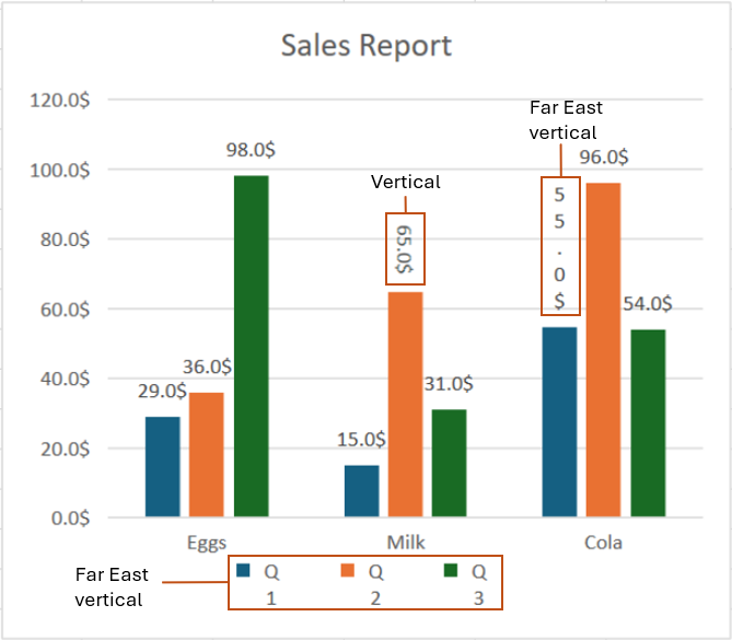
The following example demonstrates how to create a enhanced chart and set text orientation for data labels and the legend.

// Enable enhanced shape and chart engines.
fpSpread1.Features.EnhancedShapeEngine = true;
fpSpread1.Features.EnhancedChartEngine = true;

// Set data.
fpSpread1.AsWorkbook().ActiveSheet.Cells[0, 1].Value = "Eggs";
fpSpread1.AsWorkbook().ActiveSheet.Cells[0, 2].Value = "Milk";
fpSpread1.AsWorkbook().ActiveSheet.Cells[0, 3].Value = "Cola";
fpSpread1.AsWorkbook().ActiveSheet.Cells[1, 0].Value = "Q1";
fpSpread1.AsWorkbook().ActiveSheet.Cells[2, 0].Value = "Q2";
fpSpread1.AsWorkbook().ActiveSheet.Cells[3, 0].Value = "Q3";
Random random = new Random();
for (var r = 1; r <= 3; r++)
{
    for (var c = 1; c <= 3; c++)
    {
        fpSpread1.AsWorkbook().ActiveSheet.Cells[r, c].Value = 0 + random.Next(0, 100);
    }
}
fpSpread1.AsWorkbook().ActiveSheet.Cells["A1:D4"].Select();
fpSpread1.AsWorkbook().ActiveSheet.Cells["A1:D4"].NumberFormat = "0.0$";

// Add a clustered column chart.
fpSpread1.AsWorkbook().ActiveSheet.Shapes.AddChart(GrapeCity.Spreadsheet.Charts.ChartType.ColumnClustered, 100, 150, 400, 350, true);
fpSpread1.AsWorkbook().ActiveSheet.ChartObjects[0].Chart.ChartTitle.Text = "Sales Report";
fpSpread1.AsWorkbook().ActiveSheet.ChartObjects[0].Chart.ApplyDataLabels(DataLabelVisibilities.Value);

// Show the legend on the chart.
fpSpread1.AsWorkbook().ActiveSheet.ChartObjects[0].Chart.ShowLegend();
fpSpread1.AsWorkbook().ActiveSheet.ChartObjects[0].Chart.Legend.Width = 200;
fpSpread1.AsWorkbook().ActiveSheet.ChartObjects[0].Chart.Legend.Height = 60;
fpSpread1.AsWorkbook().ActiveSheet.ChartObjects[0].Chart.Series[0].ApplyDataLabels(DataLabelVisibilities.Value);

// Set data label to vertical.
fpSpread1.AsWorkbook().ActiveSheet.ChartObjects[0].Chart.Series[1].DataLabels[1].TextOrientation = TextOrientation.Vertical;

// Set data label to rotated horizontal.
fpSpread1.AsWorkbook().ActiveSheet.ChartObjects[0].Chart.Series[0].DataLabels[2].TextOrientation = TextOrientation.HorizontalRotatedFarEast;

// Set legend text to rotated horizontal.
fpSpread1.AsWorkbook().ActiveSheet.ChartObjects[0].Chart.Legend.TextOrientation = TextOrientation.HorizontalRotatedFarEast;

' Enable enhanced shape and chart engines.
fpSpread1.Features.EnhancedShapeEngine = True
fpSpread1.Features.EnhancedChartEngine = True

' Set data.
fpSpread1.AsWorkbook().ActiveSheet.Cells(0, 1).Value = "Eggs"
fpSpread1.AsWorkbook().ActiveSheet.Cells(0, 2).Value = "Milk"
fpSpread1.AsWorkbook().ActiveSheet.Cells(0, 3).Value = "Cola"
fpSpread1.AsWorkbook().ActiveSheet.Cells(1, 0).Value = "Q1"
fpSpread1.AsWorkbook().ActiveSheet.Cells(2, 0).Value = "Q2"
fpSpread1.AsWorkbook().ActiveSheet.Cells(3, 0).Value = "Q3"
Dim random As New Random()
For r As Integer = 1 To 3
    For c As Integer = 1 To 3
        fpSpread1.AsWorkbook().ActiveSheet.Cells(r, c).Value = 0 + random.Next(0, 100)
    Next
Next
fpSpread1.AsWorkbook().ActiveSheet.Cells("A1:D4").Select()
fpSpread1.AsWorkbook().ActiveSheet.Cells("A1:D4").NumberFormat = "0.0$"

' Add a clustered column chart.
fpSpread1.AsWorkbook().ActiveSheet.Shapes.AddChart(GrapeCity.Spreadsheet.Charts.ChartType.ColumnClustered, 100, 150, 400, 350, True)
fpSpread1.AsWorkbook().ActiveSheet.ChartObjects(0).Chart.ChartTitle.Text = "Sales Report"
fpSpread1.AsWorkbook().ActiveSheet.ChartObjects(0).Chart.ApplyDataLabels(DataLabelVisibilities.Value)

' Show the legend on the chart.
fpSpread1.AsWorkbook().ActiveSheet.ChartObjects(0).Chart.ShowLegend()
fpSpread1.AsWorkbook().ActiveSheet.ChartObjects(0).Chart.Legend.Width = 200
fpSpread1.AsWorkbook().ActiveSheet.ChartObjects(0).Chart.Legend.Height = 60
fpSpread1.AsWorkbook().ActiveSheet.ChartObjects(0).Chart.Series(0).ApplyDataLabels(DataLabelVisibilities.Value)

' Set data label to vertical.
fpSpread1.AsWorkbook().ActiveSheet.ChartObjects(0).Chart.Series(1).DataLabels(1).TextOrientation = TextOrientation.Vertical

' Set data label to rotated horizontal.
fpSpread1.AsWorkbook().ActiveSheet.ChartObjects(0).Chart.Series(0).DataLabels(2).TextOrientation = TextOrientation.HorizontalRotatedFarEast

' Set legend text to rotated horizontal.
fpSpread1.AsWorkbook().ActiveSheet.ChartObjects(0).Chart.Legend.TextOrientation = TextOrientation.HorizontalRotatedFarEast

Data Label Number Format

You can customize the display format for enhanced chart data labels and control whether they automatically use the number format of the source cell.

The NumberFormat property of the IDataLabel interface allows you to specify how numeric values are displayed in enhanced chart data labels. By setting this property, you can format data labels as currency, percentages, numbers with thousands separators, or include custom prefixes and suffixes.

For example, you can use #,##0,K;0 to display values in thousands with a "K" suffix, or 0.00% to display values as percentages.

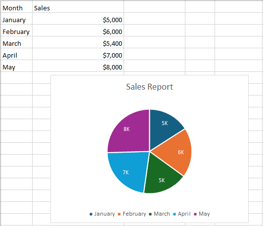
The NumberFormatLinked property determines whether the data label’s number format is linked to the source cell’s format. Set to true to automatically use the source cell’s number format; set to false to use the custom number format.

The following example demonstrates how to set a custom number format for data labels in an enhanced chart.

// Enable enhanced shape and chart engines.
fpSpread1.Features.EnhancedShapeEngine = true;
fpSpread1.Features.EnhancedChartEngine = true;

// Set data.
fpSpread1.Sheets[0].Cells[0, 0].Text = "Month";
fpSpread1.Sheets[0].Cells[0, 1].Text = "Sales";
fpSpread1.Sheets[0].Cells[1, 0].Text = "January";
fpSpread1.Sheets[0].Cells[1, 1].Value = 5000;
fpSpread1.Sheets[0].Cells[2, 0].Text = "February";
fpSpread1.Sheets[0].Cells[2, 1].Value = 6000;
fpSpread1.Sheets[0].Cells[3, 0].Text = "March";
fpSpread1.Sheets[0].Cells[3, 1].Value = 5400;
fpSpread1.Sheets[0].Cells[4, 0].Text = "April";
fpSpread1.Sheets[0].Cells[4, 1].Value = 7000;
fpSpread1.Sheets[0].Cells[5, 0].Text = "May";
fpSpread1.Sheets[0].Cells[5, 1].Value = 8000;

// Set Sales column to currency format.
fpSpread1.Sheets[0].AsWorksheet().Cells[1, 1, 5, 1].NumberFormat = "$#,##0";

fpSpread1.Sheets[0].SetActiveCell(1, 0);
fpSpread1.Sheets[0].AddSelection(1, 0, 5, 2);

// Add a pie chart.
fpSpread1.AsWorkbook().ActiveSheet.Shapes.AddChart(GrapeCity.Spreadsheet.Charts.ChartType.Pie, 100, 150, 400, 300, false);
var chart = fpSpread1.AsWorkbook().ActiveSheet.ChartObjects[0].Chart;
chart.ApplyDataLabels(DataLabelVisibilities.Value);
chart.ChartTitle.Text = "Sales Report";

// Set custom number format for data labels.
chart.Series[0].DataLabels.NumberFormat = "#,##0,K;0";
chart.Series[0].DataLabels.Format.TextFrame.TextRange.Font.Fill.BackColor.ARGB = System.Drawing.Color.White.ToArgb();

// Link data label format to source cell format (uncomment if needed).
//chart.Series[0].DataLabels.NumberFormatLinked = true;

' Enable enhanced shape and chart engines.
fpSpread1.Features.EnhancedShapeEngine = True
fpSpread1.Features.EnhancedChartEngine = True

' Set data
fpSpread1.Sheets(0).Cells(0, 0).Text = "Month"
fpSpread1.Sheets(0).Cells(0, 1).Text = "Sales"
fpSpread1.Sheets(0).Cells(1, 0).Text = "January"
fpSpread1.Sheets(0).Cells(1, 1).Value = 5000
fpSpread1.Sheets(0).Cells(2, 0).Text = "February"
fpSpread1.Sheets(0).Cells(2, 1).Value = 6000
fpSpread1.Sheets(0).Cells(3, 0).Text = "March"
fpSpread1.Sheets(0).Cells(3, 1).Value = 5400
fpSpread1.Sheets(0).Cells(4, 0).Text = "April"
fpSpread1.Sheets(0).Cells(4, 1).Value = 7000
fpSpread1.Sheets(0).Cells(5, 0).Text = "May"
fpSpread1.Sheets(0).Cells(5, 1).Value = 8000

' Set Sales column to currency format.
fpSpread1.Sheets(0).AsWorksheet().Cells(1, 1, 5, 1).NumberFormat = "$#,##0"

fpSpread1.Sheets(0).SetActiveCell(1, 0)
fpSpread1.Sheets(0).AddSelection(1, 0, 5, 2)

' Add a pie chart.
fpSpread1.AsWorkbook().ActiveSheet.Shapes.AddChart(GrapeCity.Spreadsheet.Charts.ChartType.Pie, 100, 150, 400, 300, False)
Dim chart = fpSpread1.AsWorkbook().ActiveSheet.ChartObjects(0).Chart
chart.ApplyDataLabels(DataLabelVisibilities.Value)
chart.ChartTitle.Text = "Sales Report"

' Set custom number format for data labels.
chart.Series(0).DataLabels.NumberFormat = "#,##0,K;0"
chart.Series[0].DataLabels.Format.TextFrame.TextRange.Font.Fill.BackColor.ARGB = System.Drawing.Color.White.ToArgb()

' Link data label format to source cell format (uncomment if needed).
'chart.Series(0).DataLabels.NumberFormatLinked = True

Set Label Position

The IDataLabel.DataLabelPosition property allows users to flexibly set the position of data labels on the enhanced chart, similar to Microsoft Excel. Available options include Center, Inside End, Outside End, Inside Base, Top, Bottom, Left, Right, and Best Fit.

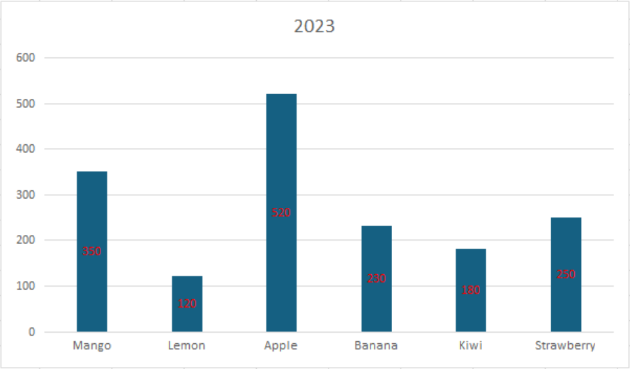
The following example demonstrates how to set the label position of an enhanced chart to Center.

// Enable enhanced shape and chart engines.
fpSpread1.Features.EnhancedShapeEngine = true;
fpSpread1.Features.EnhancedChartEngine = true;

// Set data.
object[,] values = new object[,]
{
    {null,"Mango","Lemon","Apple","Banana","Kiwi","Strawberry"},
    {2023, 350,120,520,230,180,250 },
};
fpSpread1.AsWorkbook().ActiveSheet.SetValue(0, 0, values, false);
fpSpread1.AsWorkbook().ActiveSheet.Cells["A1:G2"].Select();

// Add a clustered column chart.
fpSpread1.AsWorkbook().ActiveSheet.Shapes.AddChart(ChartType.ColumnClustered, 100, 150, 600, 350);
fpSpread1.AsWorkbook().ActiveSheet.ChartObjects[0].Chart.ApplyDataLabels(DataLabelVisibilities.Value);

// Set the position of data labels to Center.
fpSpread1.AsWorkbook().ActiveSheet.ChartObjects[0].Chart.Series[0].DataLabels.Position = DataLabelPosition.Center;
fpSpread1.AsWorkbook().ActiveSheet.ChartObjects[0].Chart.Series[0].DataLabels.Format.TextFrame.TextRange.Font.Fill.BackColor.ARGB = System.Drawing.Color.Red.ToArgb();

' Enable enhanced shape and chart engines.
fpSpread1.Features.EnhancedShapeEngine = True
fpSpread1.Features.EnhancedChartEngine = True

' Set data.
Dim values As Object(,) = {
    {Nothing, "Mango", "Lemon", "Apple", "Banana", "Kiwi", "Strawberry"},
    {2023, 350, 120, 520, 230, 180, 250}
}
fpSpread1.AsWorkbook().ActiveSheet.SetValue(0, 0, values, False)
fpSpread1.AsWorkbook().ActiveSheet.Cells("A1:G2").Select()

' Add a clustered column chart.
fpSpread1.AsWorkbook().ActiveSheet.Shapes.AddChart(ChartType.ColumnClustered, 100, 150, 600, 350)
fpSpread1.AsWorkbook().ActiveSheet.ChartObjects(0).Chart.ApplyDataLabels(DataLabelVisibilities.Value)

' Set the position of data labels to Center.
fpSpread1.AsWorkbook().ActiveSheet.ChartObjects(0).Chart.Series(0).DataLabels.Position = DataLabelPosition.Center
fpSpread1.AsWorkbook().ActiveSheet.ChartObjects(0).Chart.Series(0).DataLabels.Format.TextFrame.TextRange.Font.Fill.BackColor.ARGB = System.Drawing.Color.Red.ToArgb()

Auto-size Data Labels

The IDataLabel.AutoText property gets or sets a value indicating whether the enhanced chart data label automatically generates appropriate text and resizes itself based on context. When enabled, the data label adjusts its size to display the complete text without clipping.

AutoText Disabled	AutoText Enabled

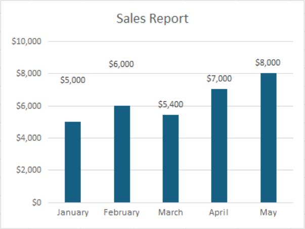
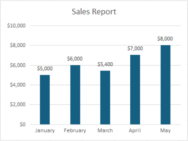
The following example demonstrates how to enable auto-size data labels in a clustered column chart.

// Enable enhanced shape and chart engines.
fpSpread1.Features.EnhancedShapeEngine = true;
fpSpread1.Features.EnhancedChartEngine = true;

// Set data.
fpSpread1.Sheets[0].Cells[0, 0].Text = "Month";
fpSpread1.Sheets[0].Cells[0, 1].Text = "Sales";
fpSpread1.Sheets[0].Cells[1, 0].Text = "January";
fpSpread1.Sheets[0].Cells[1, 1].Value = 5000;
fpSpread1.Sheets[0].Cells[2, 0].Text = "February";
fpSpread1.Sheets[0].Cells[2, 1].Value = 6000;
fpSpread1.Sheets[0].Cells[3, 0].Text = "March";
fpSpread1.Sheets[0].Cells[3, 1].Value = 5400;
fpSpread1.Sheets[0].Cells[4, 0].Text = "April";
fpSpread1.Sheets[0].Cells[4, 1].Value = 7000;
fpSpread1.Sheets[0].Cells[5, 0].Text = "May";
fpSpread1.Sheets[0].Cells[5, 1].Value = 8000;

// Set Sales column to currency format.
fpSpread1.Sheets[0].AsWorksheet().Cells[1, 1, 5, 1].NumberFormat = "$#,##0";
fpSpread1.Sheets[0].SetActiveCell(1, 0);
fpSpread1.Sheets[0].AddSelection(1, 0, 5, 2);

// Add a pie chart.
fpSpread1.AsWorkbook().ActiveSheet.Shapes.AddChart(GrapeCity.Spreadsheet.Charts.ChartType.ColumnClustered, 100, 150, 400, 300);
var chart = fpSpread1.AsWorkbook().ActiveSheet.ChartObjects[0].Chart;
chart.ApplyDataLabels(DataLabelVisibilities.Value);
chart.ChartTitle.Text = "Sales Report";

// Enable auto-size for all data labels in the series.
fpSpread1.AsWorkbook().ActiveSheet.ChartObjects[0].Chart.Series[0].DataLabels[0].Height = 100;
fpSpread1.AsWorkbook().ActiveSheet.ChartObjects[0].Chart.Series[0].DataLabels[1].Height = 100;
fpSpread1.AsWorkbook().ActiveSheet.ChartObjects[0].Chart.Series[0].DataLabels.Format.TextFrame.AutoSize = true;

' Enable enhanced shape and chart engines.
FpSpread1.Features.EnhancedShapeEngine = True
FpSpread1.Features.EnhancedChartEngine = True

' Set data.
FpSpread1.Sheets(0).Cells(0, 0).Text = "Month"
FpSpread1.Sheets(0).Cells(0, 1).Text = "Sales"
FpSpread1.Sheets(0).Cells(1, 0).Text = "January"
FpSpread1.Sheets(0).Cells(1, 1).Value = 5000
FpSpread1.Sheets(0).Cells(2, 0).Text = "February"
FpSpread1.Sheets(0).Cells(2, 1).Value = 6000
FpSpread1.Sheets(0).Cells(3, 0).Text = "March"
FpSpread1.Sheets(0).Cells(3, 1).Value = 5400
FpSpread1.Sheets(0).Cells(4, 0).Text = "April"
FpSpread1.Sheets(0).Cells(4, 1).Value = 7000
FpSpread1.Sheets(0).Cells(5, 0).Text = "May"
FpSpread1.Sheets(0).Cells(5, 1).Value = 8000

' Set Sales column to currency format.
FpSpread1.Sheets(0).AsWorksheet().Cells(1, 1, 5, 1).NumberFormat = "$#,##0"
FpSpread1.Sheets(0).SetActiveCell(1, 0)
FpSpread1.Sheets(0).AddSelection(1, 0, 5, 2)

' Add a clustered column chart.
FpSpread1.AsWorkbook().ActiveSheet.Shapes.AddChart(GrapeCity.Spreadsheet.Charts.ChartType.ColumnClustered, 100, 150, 400, 300)
Dim chart = FpSpread1.AsWorkbook().ActiveSheet.ChartObjects(0).Chart
chart.ApplyDataLabels(DataLabelVisibilities.Value)
chart.ChartTitle.Text = "Sales Report"

' Enable auto-size for all data labels in the series.
FpSpread1.AsWorkbook().ActiveSheet.ChartObjects(0).Chart.Series(0).DataLabels(0).Height = 100
FpSpread1.AsWorkbook().ActiveSheet.ChartObjects(0).Chart.Series(0).DataLabels(1).Height = 100
FpSpread1.AsWorkbook().ActiveSheet.ChartObjects(0).Chart.Series(0).DataLabels.Format.TextFrame.AutoSize = True