
Conditional Formatting
Spread for WPF allows you to apply conditional formatting rules to worksheet cells. This feature enhances data visualization and helps you analyze worksheets. To apply conditional formatting rules to a worksheet, you can use the properties and methods of the IFormatConditions interface.
Here are some basic conditions regarding the rules for the conditional formatting:
Conditional formatting rules work based on a predefined order of precedence, where the last rule in the list has the highest precedence.
By default, new rules are always added to the last and therefore possess the highest precedence.
If a conflict occurs between two rules, the rule with the higher precedence is applied.
If two rules do not conflict, then both the rules are applied.
For example, consider a rule that defines a bold font and another that sets cell background color. In this case, both rules will be applied.
There are multiple types of conditional rules. The following sections outline these rules along with their explanations.
Color Scales Rule
Color scales rule is useful to represent values in a range of cells as high, medium, or low using different shades. This rule uses a sliding color scale and gives you the option to use two colors (2-scale rule) or three colors (3-scale rule) in the scale. For example, consider a green, yellow, and red color scale where you can specify higher values with green color, middle values with yellow color, and lower values with red color.
To apply a color scale rule, you can use the AddColorScale method of the IFormatConditions interface. When you define a color scale rule, you can specify the format type using the Numeric field of the CfValueType enumeration and the color of the format using the IsKnownColor method of the Color structure along with the KnownColor enumeration.
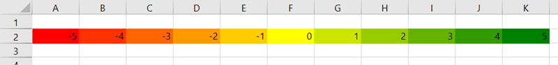
The following code sample creates a color scale rule.
C#
// Color scale rule.
GrapeCity.Spreadsheet.IColorScale colorScale = spreadSheet1.Workbook.ActiveSheet.Range("A2:K2").FormatConditions.AddColorScale(3); // Use 3 color levels
colorScale.ColorScaleCriteria[0].Type = GrapeCity.Spreadsheet.CfValueType.Numeric;
colorScale.ColorScaleCriteria[0].Value = -5; // Set a negative value
colorScale.ColorScaleCriteria[0].FormatColor = GrapeCity.Spreadsheet.Color.FromKnownColor(GrapeCity.Core.KnownColor.Red);
colorScale.ColorScaleCriteria[1].Type = GrapeCity.Spreadsheet.CfValueType.Numeric;
colorScale.ColorScaleCriteria[1].Value = 0;
colorScale.ColorScaleCriteria[1].FormatColor = GrapeCity.Spreadsheet.Color.FromKnownColor(GrapeCity.Core.KnownColor.Yellow);
colorScale.ColorScaleCriteria[2].Type = GrapeCity.Spreadsheet.CfValueType.Numeric;
colorScale.ColorScaleCriteria[2].Value = 5; // Set a positive value
colorScale.ColorScaleCriteria[2].FormatColor = GrapeCity.Spreadsheet.Color.FromKnownColor(GrapeCity.Core.KnownColor.Green);
for (int i = 0; i < 11; i++)
{
  spreadSheet1.Workbook.ActiveSheet.Cells[1, i].Value = i - 5;
}
VB
' Color scale rule.
Dim colorScale As GrapeCity.Spreadsheet.IColorScale = spreadSheet1.Workbook.ActiveSheet.Range("A2:K2").FormatConditions.AddColorScale(3) ' Use 3 color levels
colorScale.ColorScaleCriteria(0).Type = GrapeCity.Spreadsheet.CfValueType.Numeric
colorScale.ColorScaleCriteria(0).Value = -5 ' Set a negative value
colorScale.ColorScaleCriteria(0).FormatColor = GrapeCity.Spreadsheet.Color.FromKnownColor(GrapeCity.Core.KnownColor.Red)
colorScale.ColorScaleCriteria(1).Type = GrapeCity.Spreadsheet.CfValueType.Numeric
colorScale.ColorScaleCriteria(1).Value = 0
colorScale.ColorScaleCriteria(1).FormatColor = GrapeCity.Spreadsheet.Color.FromKnownColor(GrapeCity.Core.KnownColor.Yellow)
colorScale.ColorScaleCriteria(2).Type = GrapeCity.Spreadsheet.CfValueType.Numeric
colorScale.ColorScaleCriteria(2).Value = 5 ' Set a positive value
colorScale.ColorScaleCriteria(2).FormatColor = GrapeCity.Spreadsheet.Color.FromKnownColor(GrapeCity.Core.KnownColor.Green)
For i = 0 To 10
  spreadSheet1.Workbook.ActiveSheet.Cells(1, i).Value = i - 5
Next
Data Bars Rule
Data bars rule displays a bar in a cell based on the cell value. The length of the data bar matches the size of the data that is related to other data in the worksheet. The larger the value in the cell, the longer the bar.
To apply a data bar rule, you can use the AddDatabar method of the IFormatConditions interface. When defining a data bar rule, you can specify the color of the data bar using the FromArgb method of the Color structure and the color type using the DatabarNegativeColorType enumeration. To set the axis position, you can use the AxisPosition property of the IDatabar interface.
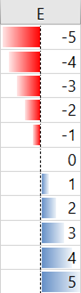
The following code sample creates a data bar rule.
C#
// Data bar rule.
GrapeCity.Spreadsheet.IDatabar databar = spreadSheet1.Workbook.ActiveSheet.Range("E1:E11").FormatConditions.AddDatabar();
databar.NegativeBarFormat.Color = GrapeCity.Spreadsheet.Color.FromArgb(255, 0, 0);
databar.NegativeBarFormat.ColorType = GrapeCity.Spreadsheet.DatabarNegativeColorType.Color;
databar.AxisPosition = GrapeCity.Spreadsheet.DatabarAxisPosition.Middle;
for (int i = 0; i < 11; i++)
{
    spreadSheet1.Workbook.ActiveSheet.Cells[i, 4].Value = i - 5;
}
VB
' Data bar rule.
Dim databar As GrapeCity.Spreadsheet.IDatabar = spreadSheet1.Workbook.ActiveSheet.Range("E1:E11").FormatConditions.AddDatabar()
databar.NegativeBarFormat.Color = GrapeCity.Spreadsheet.Color.FromArgb(255, 0, 0)
databar.NegativeBarFormat.ColorType = GrapeCity.Spreadsheet.DatabarNegativeColorType.Color
databar.AxisPosition = GrapeCity.Spreadsheet.DatabarAxisPosition.Middle
For i = 0 To 10
   spreadSheet1.Workbook.ActiveSheet.Cells(i, 4).Value = i - 5
Next
Highlight Cells Rule
Highlighting rules can be applied in a worksheet to emphasize relevant information. You can highlight data by either applying a predefined style from the following list of data highlighting rules or creating a custom highlight style as per your specific preferences.
You can highlight data which is:
Greater than a particular value.
Less than a particular value.
Between a high and low value.
Equal to a particular value.
Data that contains a specific value.
Data that contains a date that occurs in a particular range.
Data which is either unique or duplicated elsewhere in the worksheet.
To apply highlighting rules in a worksheet, you can set any one of the above condition by using the AddUniqueValues method of the IFormatConditions interface. Next, you need to enter a value or formula against which each cell is compared and then the formatting is applied based on the cell data that satisfies the specified criteria.
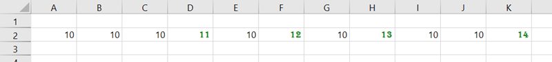
The following code sample creates a highlighting cell rule.
C#
// Highlight cell rule.
GrapeCity.Spreadsheet.IUniqueValues uniqueValues = spreadSheet1.Workbook.ActiveSheet.Range("A2:K2").FormatConditions.AddUniqueValues();
uniqueValues.DupeUnique = GrapeCity.Spreadsheet.DupeUnique.Unique;
uniqueValues.Font.Color = GrapeCity.Spreadsheet.Color.FromKnownColor(GrapeCity.Core.KnownColor.Green);
uniqueValues.Font.Name = "Algerian";
uniqueValues.Font.Superscript = true;
for (int i = 0; i < 11; i++)
{
    spreadSheet1.Workbook.ActiveSheet.Cells[1, i].Value = 10;
}
spreadSheet1.Workbook.ActiveSheet.Cells[1, 3].Value = 11;
spreadSheet1.Workbook.ActiveSheet.Cells[1, 5].Value = 12;
spreadSheet1.Workbook.ActiveSheet.Cells[1, 7].Value = 13;
spreadSheet1.Workbook.ActiveSheet.Cells[1, 10].Value = 14;
VB
' Highlight cell rule.
Dim uniqueValues As GrapeCity.Spreadsheet.IUniqueValues = spreadSheet1.Workbook.ActiveSheet.Range("A2:K2").FormatConditions.AddUniqueValues()
uniqueValues.DupeUnique = GrapeCity.Spreadsheet.DupeUnique.Unique
uniqueValues.Font.Color = GrapeCity.Spreadsheet.Color.FromKnownColor(GrapeCity.Core.KnownColor.Green)
uniqueValues.Font.Name = "Algerian"
uniqueValues.Font.Superscript = True
For i = 0 To 10
   spreadSheet1.Workbook.ActiveSheet.Cells(1, i).Value = 10
Next
spreadSheet1.Workbook.ActiveSheet.Cells(1, 3).Value = 11
spreadSheet1.Workbook.ActiveSheet.Cells(1, 5).Value = 12
spreadSheet1.Workbook.ActiveSheet.Cells(1, 7).Value = 13
spreadSheet1.Workbook.ActiveSheet.Cells(1, 10).Value = 14
Icon Sets Rule
Icon set rule displays custom icons when the value of a cell is greater than, equal to, or less than the specified value.
To apply icon set rule in a worksheet, you can use the AddIconSetCondition method of the IFormatConditions interface. You can specify the icon set type by using the IconSetType enumeration and then use the methods and properties of the IIconCriteria interface to specify the criteria for applying the icon set rule.

The following code sample creates an icon set rule.
C#
// Icon set rule.
GrapeCity.Spreadsheet.IIconSetCondition iconSet =
spreadSheet1.Workbook.ActiveSheet.Range("A2:K2").FormatConditions.AddIconSetCondition();
iconSet.IconSet = GrapeCity.Spreadsheet.IconSetType.ThreeSymbols;
iconSet.IconCriteria[1].Operator = GrapeCity.Spreadsheet.Operator.GreaterThanOrEqual;
iconSet.IconCriteria[1].Value = 50;
iconSet.IconCriteria[1].Type = GrapeCity.Spreadsheet.CfValueType.Percent;
iconSet.IconCriteria[2].Operator = GrapeCity.Spreadsheet.Operator.GreaterThanOrEqual;
iconSet.IconCriteria[2].Value = 70;
iconSet.IconCriteria[2].Type = GrapeCity.Spreadsheet.CfValueType.Percent;
for (int i = 0; i < 11; i++)
{
    spreadSheet1.Workbook.ActiveSheet.Cells[1, i].Value = i - 5;
}
VB
' Icon set rule.
Dim iconSet As GrapeCity.Spreadsheet.IIconSetCondition = spreadSheet1.Workbook.ActiveSheet.Range("A2:K2").FormatConditions.AddIconSetCondition()
iconSet.IconSet = GrapeCity.Spreadsheet.IconSetType.ThreeSymbols
iconSet.IconCriteria(1).[Operator] = GrapeCity.Spreadsheet.[Operator].GreaterThanOrEqual
iconSet.IconCriteria(1).Value = 50
iconSet.IconCriteria(1).Type = GrapeCity.Spreadsheet.CfValueType.Percent
iconSet.IconCriteria(2).[Operator] = GrapeCity.Spreadsheet.[Operator].GreaterThanOrEqual
iconSet.IconCriteria(2).Value = 70
iconSet.IconCriteria(2).Type = GrapeCity.Spreadsheet.CfValueType.Percent
For i = 0 To 10
    spreadSheet1.Workbook.ActiveSheet.Cells(1, i).Value = i - 5
Next
Top/Bottom/Average Rule
Top/Bottom rules apply formatting to cells whose values are within the top or bottom 10 percent. The Top10 rule uses the TopBottom enumeration to specify the top or bottom values. You can also change the percentage using the Rank property of the ITop10 interface. Additionally, the average rule checks for values that are either above the average value or below the average value. This rule applies formatting to the greater or lesser average value of the entire range.
To apply top, bottom or average rule, you can use the AddTop10 method and the AddAboveAverage method of the IFormatConditions interface.

The following code sample creates a rule to identify the top 50 percent of the values.
C#
// Top, bottom, average rules (apply formatting to the top 50 percent of values in A2:K2)
GrapeCity.Spreadsheet.ITop10 top10Set =
spreadSheet1.Workbook.ActiveSheet.Range("A2:K2").FormatConditions.AddTop10();
top10Set.TopBottom = GrapeCity.Spreadsheet.TopBottom.Top10Top;
top10Set.Rank = 50;
top10Set.Percent = true;
top10Set.Interior.Color = GrapeCity.Spreadsheet.Color.FromKnownColor(GrapeCity.Core.KnownColor.Aqua);
for (int col = 0; col < 11; col++)
{
     spreadSheet1.Workbook.ActiveSheet.Cells[1, col].Value = col - 5;
}
VB
' Top, bottom, average rules (apply formatting to the top 50 percent of values in A2:K2)
Dim top10Set As GrapeCity.Spreadsheet.ITop10 = spreadSheet1.Workbook.ActiveSheet.Range("A2:K2").FormatConditions.AddTop10()
top10Set.TopBottom = GrapeCity.Spreadsheet.TopBottom.Top10Top
top10Set.Rank = 50
top10Set.Percent = True
top10Set.Interior.Color = GrapeCity.Spreadsheet.Color.FromKnownColor(GrapeCity.Core.KnownColor.Aqua)
For col = 0 To 10
   spreadSheet1.Workbook.ActiveSheet.Cells(1, col).Value = col - 5
Next