
- Spread for WPF Overview
- About the Product
- Getting Started
- Quick Start
- Designer
- Features
- Assembly Reference
Cells
A cell is the basic unit of a worksheet, which is formed at the intersection of a row and a column. Spread for WPF lets you work with cells and perform different operations on them, as explained in the following sections.
Set Active Cell
Active cell refers to the currently selected or highlighted cell into which data is being entered when you start typing. Only one cell is active at a time. By default, A1 is the active cell and it is displayed with a thick border. You can also move the active cell by clicking on any other cell.
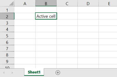
To set your desired cell as an active cell, use the Activate() method of the IRange interface. This method is called to set particular cell as active cell.
Refer to the following example code to set the B2 cell as the active cell.
C#
// Set active cell.
spreadSheet1.Workbook.ActiveSheet.Cells["B2"].Activate();
spreadSheet1.Workbook.ActiveSheet.ActiveCell.Value = "Active cell";
VB
' Set active cell.
spreadSheet1.Workbook.ActiveSheet.Cells("B2").Activate()
spreadSheet1.Workbook.ActiveSheet.ActiveCell.Value = "Active cell"
Focus the Active Cell
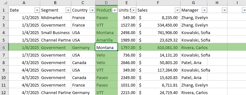
Focusing the active cell enhances its visibility by highlighting the corresponding row and column. This feature improves navigation and readability, especially when working with large datasets.
Spread WPF implements the active cell focus through the FocusCellMode setting. It is enabled only when a valid active cell exists. If the current selection configuration does not maintain an active cell, the active cell will not be rendered as the focus cell.
When the active cell is focused:
The value of the active cell remains unchanged.
The row and/or column of the active cell is visually highlighted based on the FocusCellMode setting.
The highlight updates dynamically as the active cell changes.
The highlight is rendered as a UI overlay and does not modify conditional formatting.
This feature does not affect selection behavior or editing.
If the active cell is a merged cell, the highlight extends to all rows and columns in the merged range.
Spread WPF provides the FocusCellMode enumeration to specify how the active cell is highlighted. When set to Row or Column, it highlights the active cell’s row or column respectively. When set to Both, both the row and column are highlighted.
Refer to the following example code that shows how to focus active cell in both XAML view and in the code view.
XAML
<Grid>
    <gss:GcSpreadSheet x:Name="GcSpreadSheet1"  FocusCellMode="Both" />
</Grid>
C#
// Set focus mode to highlight both the row and column of the active cell.
GcSpreadSheet1.FocusCellMode = GrapeCity.Wpf.SpreadSheet.FocusCellMode.Both;

// Activate cell D5 on the active sheet.
GcSpreadSheet1.Workbook.ActiveSheet.Cells["D6"].Activate();

// Set the focus cell highlight color.
GcSpreadSheet1.FocusCellColor = GrapeCity.Core.SchemeColor.CreateArgbColor(166, 211, 150, 255);
VB
' Set focus mode to highlight both the row and column of the active cell.
GcSpreadSheet1.FocusCellMode = GrapeCity.Wpf.SpreadSheet.FocusCellMode.Both

' Activate cell D5 on the active sheet.
GcSpreadSheet1.Workbook.ActiveSheet.Cells("D6").Activate()

' Set the focus cell highlight color.
GcSpreadSheet1.FocusCellColor = GrapeCity.Core.SchemeColor.CreateArgbColor(166, 211, 150, 255)
Merge Cells
You can merge the cells in a worksheet to span multiple rows or columns. Merging cells allows you to combine multiple cells in a worksheet into a single large cell. This is useful when you want to organize or format your worksheet content.
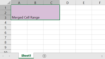
When you merge cells, the data of the first cell (the "anchor cell") in the range will expand to fill all the merged space. The data in the other cells in the range will be hidden, but not lost. Once you unmerge the cells, the hidden data will reappear as before. For example, if the cell range A1 to C3 has the same value, you can merge them and then the cell A1 will occupy the space from A1 to C3 as shown in the following image.
To merge and unmerge the cells in a worksheet, use the Merge and UnMerge methods of the IRange interface.
Refer to the following example code that merges the cell A1:C3 and creates a single merged cell and unmerge it later.
C#
// Merge cells.
spreadSheet1.Workbook.ActiveSheet.Cells["A1"].Interior.Color = GrapeCity.Spreadsheet.Color.FromKnownColor(GrapeCity.Core.KnownColor.Thistle);
spreadSheet1.Workbook.ActiveSheet.Cells["A1:C3"].Merge();
spreadSheet1.Workbook.ActiveSheet.Cells["A1"].Text = "Merged Cell Range";
// Unmerge cells.
spreadSheet1.Workbook.ActiveSheet.Cells["A1:C3"].UnMerge();
VB
' Merge cells.
spreadSheet1.Workbook.ActiveSheet.Cells("A1").Interior.Color = GrapeCity.Spreadsheet.Color.FromKnownColor(GrapeCity.Core.KnownColor.Thistle)
spreadSheet1.Workbook.ActiveSheet.Cells("A1:C3").Merge()
spreadSheet1.Workbook.ActiveSheet.Cells("A1").Text = "Merged Cell Range"
' Unmerge cells.
spreadSheet1.Workbook.ActiveSheet.Cells("A1:C3").UnMerge()
Merge Priority Rules
When merging cells, if the range overlaps with another merged range, the merge range shown in the control will be determined by the merge range priority. The priority of the merging range is decided based on the rules listed below.
The row with the smallest index of the cell in the combined range takes priority.
For the same row index, the column with the smaller index takes priority.
Auto-Merge Cells
The Auto-Merge feature simplifies the process of merging duplicate content in adjacent cells. It automatically merges rows or columns with the same value. This helps you remove redundancies (repeated text) and reduce the complexity of your worksheet. It also saves you time and effort by eliminating the need to manually check for duplicate cells and merge them one by one.
To enable automatic merging of cells in a worksheet, you can use the MergePolicy enumeration of the GrapeCity.Spreadsheet namespace. It helps to set the merge policies for the columns to control how cells can be merged. The MergePolicy has the following members:
Always: Automatically merges adjacent cells with identical values.
None: Never automatically merges cells.
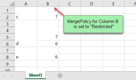
Restricted: Automatically merges adjacent cells with identical values if the corresponding cells in another row or column are similarly merged.
For example, set the value of cells A1:A8 as {c; c; d; d; d; d; e; e} and the value of cells B1:B8 as {7; 7; 7; 7; 7; 6; 6; 6}. If column B has a merge policy of "Always", the cells in column B will be merged into two blocks: B1:B5 and B6:B8. On the other hand, if column B has a merge policy of "Restricted", the cells in column B will be merged into four blocks: B1:B2, B3:B5, B6, B7:B8.
Note:
The data in the merged cells are not lost, they are just hidden.
You can edit the original content by double-clicking the cell. When you exit the edit mode, if the cell's content differs from the other cells it was merged with, the cell will no longer look as merged.
Cells of different cell types that contain same data can also be merged.
For example, a cell with a string cell type contains content "45" and the adjacent cell with a number cell type contains the same content; then both the cells will automatically be merged.
Merged cells inherit the properties of the top-left cell in the merged range.
For example, if the top-left merged cell has the red background color, all merged cells will have the same background color.
Refer to the following example code that shows how to auto-merge cells with the same values in the second column in a worksheet in both XAML view and in the code view.
XAML
<gss:GcSpreadSheet Name="spreadSheet1" HorizontalAlignment="Left" Margin="10,24,0,0" VerticalAlignment="Top">
            <gss:GcSpreadSheet.Sheets>
                <gss:SheetInfo Name="Sheet1" RowCount="10">
                    <gss:SheetInfo.Columns>
                        <gss:ColumnInfo />
                        <gss:ColumnInfo MergePolicy ="Always"/>
                        <gss:ColumnInfo/>
                        <gss:ColumnInfo />
                        <gss:ColumnInfo/>
                        <gss:ColumnInfo/>
                    </gss:SheetInfo.Columns>
                </gss:SheetInfo>
            </gss:GcSpreadSheet.Sheets>
</gss:GcSpreadSheet>
C#
// Set MergePolicy to "Always".
spreadSheet1.Workbook.ActiveSheet.Cells["B1"].Text = "AutoMerge";
spreadSheet1.Workbook.ActiveSheet.Cells["B2"].Text = "AutoMerge";
spreadSheet1.Workbook.ActiveSheet.Cells["B3"].Text = "AutoMerge";
spreadSheet1.Workbook.ActiveSheet.Cells["B4"].Text = "AutoMerge";
spreadSheet1.Workbook.ActiveSheet.Columns[1].MergePolicy = MergePolicy.Always;
VB
' Set the MergePolicy of the second column to "Always".
spreadSheet1.Workbook.ActiveSheet.Cells("B1").Text = "AutoMerge"
spreadSheet1.Workbook.ActiveSheet.Cells("B2").Text = "AutoMerge"
spreadSheet1.Workbook.ActiveSheet.Cells("B3").Text = "AutoMerge"
spreadSheet1.Workbook.ActiveSheet.Cells("B4").Text = "AutoMerge"
spreadSheet1.Workbook.ActiveSheet.Columns(1).MergePolicy = MergePolicy.Always
Unlock Cells
Protecting a worksheet prevents its cells from being edited by default. To enable cell editing, unlock the cells by setting the Locked property of the IRange interface to false. Note that the data can be copied from locked cells.
Refer to the following example code to unlock cells to edit.
C#
// Protect worksheet.
spreadSheet1.Workbook.ActiveSheet.Protect(GrapeCity.Spreadsheet.WorksheetLocks.All, "test");
// Unlock cells.
spreadSheet1.Workbook.ActiveSheet.Cells["C3:D4"].Text = "Unlocked";
spreadSheet1.Workbook.ActiveSheet.Cells["C3:D4"].Locked = false;
VB
' Protect worksheet.
spreadSheet1.Workbook.ActiveSheet.Protect(GrapeCity.Spreadsheet.WorksheetLocks.All, "test")
' Unlock cells.
spreadSheet1.Workbook.ActiveSheet.Cells("C3:D4").Text = "Unlocked"
spreadSheet1.Workbook.ActiveSheet.Cells("C3:D4").Locked = False
Format Cell Text
You can change font settings such as font, size, style, color, etc. of the cell text using properties like Name, Size, Italic, Color, and several methods of the IFont interface. Additionally, Spread for WPF allows you to change the horizontal and vertical alignment of the cell using the HorizontalAlignment and VerticalAlignment properties of the IRange interface.
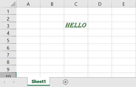
Refer to the following example code to format cell text.
C#
// Cell font.
spreadSheet1.Workbook.ActiveSheet.Cells[2, 2].Text = "Hello";
spreadSheet1.Workbook.ActiveSheet.Cells[2, 2].Font.Name = "Algerian";
spreadSheet1.Workbook.ActiveSheet.Cells[2, 2].Font.Size = 14;
spreadSheet1.Workbook.ActiveSheet.Cells[2, 2].Font.Italic = true;
spreadSheet1.Workbook.ActiveSheet.Cells[2, 2].Font.Color = GrapeCity.Spreadsheet.Color.FromThemeColor(GrapeCity.Core.ThemeColors.Accent3);
// Cell alignment.
spreadSheet1.Workbook.ActiveSheet.Cells[2, 2].HorizontalAlignment = GrapeCity.Spreadsheet.HorizontalAlignment.Center;
spreadSheet1.Workbook.ActiveSheet.Cells[2, 2].VerticalAlignment = GrapeCity.Spreadsheet.VerticalAlignment.Center;
VB
' Cell font.
spreadSheet1.Workbook.ActiveSheet.Cells(2, 2).Text = "Hello"
spreadSheet1.Workbook.ActiveSheet.Cells(2, 2).Font.Name = "Algerian"
spreadSheet1.Workbook.ActiveSheet.Cells(2, 2).Font.Size = 14
spreadSheet1.Workbook.ActiveSheet.Cells(2, 2).Font.Italic = True
spreadSheet1.Workbook.ActiveSheet.Cells[2, 2].Font.Color = GrapeCity.Spreadsheet.Color.FromThemeColor(GrapeCity.Core.ThemeColors.Accent3)
' Cell alignment.
spreadSheet1.Workbook.ActiveSheet.Cells(2, 2).HorizontalAlignment = GrapeCity.Spreadsheet.HorizontalAlignment.Center
spreadSheet1.Workbook.ActiveSheet.Cells(2, 2).VerticalAlignment = GrapeCity.Spreadsheet.VerticalAlignment.Center
Change Cell Size
You can modify the column width and row height of a worksheet to fit the data by changing the cell size. To do this, use the ColumnWidth and RowHeight properties of the IRange interface.
Refer to the following example code that changes the cell size.
C#
// Set cell size.
spreadSheet1.Workbook.ActiveSheet.Cells[2, 2].ColumnWidth = 100;
spreadSheet1.Workbook.ActiveSheet.Cells[2, 2].RowHeight = 60;
VB
' Set cell size.
spreadSheet1.Workbook.ActiveSheet.Cells(2, 2).ColumnWidth = 100
spreadSheet1.Workbook.ActiveSheet.Cells(2, 2).RowHeight = 60
Set Cell Background Color
Spread for WPF allows you to set the background colors of worksheet cells, which can help you highlight relevant data. To change the background color of a cell, use the Color property of the IInterior interface for the specified cell index.
Additionally, the mouse hover color, the background color of a cell when hovered over, can also be set using the HoverCellBackground property of the GcSpreadSheet class.
C#
// Set the cell background color.
GrapeCity.Spreadsheet.IWorksheet worksheet = spreadSheet1.Workbook.Worksheets[0];
worksheet.Cells[0, 0].Value = 123;
worksheet.Cells[0, 0].Interior.Color = GrapeCity.Spreadsheet.Color.FromKnownColor(GrapeCity.Core.KnownColor.Red);
// Set the mouse hover color.
spreadSheet1.HoverCellBackground = new SolidColorBrush(System.Windows.Media.Color.FromArgb(128, 0, 255, 255));
VB
' Set the cell background color.
Dim worksheet As GrapeCity.Spreadsheet.IWorksheet = spreadSheet1.Workbook.Worksheets(0)
worksheet.Cells(0, 0).Value = 123
worksheet.Cells(0, 0).Interior.Color = GrapeCity.Spreadsheet.Color.FromKnownColor(GrapeCity.Core.KnownColor.Red)
' Set the mouse hover color.
spreadSheet1.HoverCellBackground = New SolidColorBrush(Windows.Media.Color.FromArgb(128, 0, 255, 255))
You can also set the background color of active or selected cell by using the SelectionBackground or ActiveCellBackground property of GcSpreadSheet class. To do this, make sure that you have set the SelectionStyle property that indicates how the selection is painted. This property has the following values:
Value | Description |
|---|---|
None | Does not change the style of selected cells. |
Renderer | Uses default color for selected cells (transparent grey for selection, and white for active cell). |
Color | Uses the selected background color for selected cells. |
Both | Uses both the selected background color and renderer for selected cells. |
The following example code shows how to set the background color of the active or selected cell in both XAML view and in the code view.
XAML
< gss:GcSpreadSheet x:Name ="spreadSheet1" SelectionStyle ="Both" SelectionBackground ="LightPink" ActiveCellBackground ="LightYellow" />C#
// Set SelectionStyle to "Both".
spreadSheet1.SelectionStyle = SelectionStyle.Both;
// Set the ActiveCellBackground.
spreadSheet1.ActiveCellBackground = System.Windows.Media.Brushes.LightYellow;
// Set SelectionBackground.
spreadSheet1.SelectionBackground = System.Windows.Media.Brushes.LightPink;
VB
' Set SelectionStyle to "Both".
spreadSheet1.SelectionStyle = SelectionStyle.Both
' Set the ActiveCellBackground.
spreadSheet1.ActiveCellBackground = Windows.Media.Brushes.LightYellow
' Set SelectionBackground.
spreadSheet1.SelectionBackground = Windows.Media.Brushes.LightPink
Customize Cell Borders
You can set worksheet cell borders using the ApplyBorder method of the IBorders interface. It method allows you to change the color and line style of cell borders. However, you can use the BordersIndex enumeration if you want to explicitly set the style for one side of a border.
Refer to the following example code to change cell borders.
C#
// Set cell borders.
spreadSheet1.Workbook.ActiveSheet.Cells[4, 2].Borders.ApplyBorder(new GrapeCity.Spreadsheet.Border
(new GrapeCity.Spreadsheet.BorderLine(GrapeCity.Spreadsheet.BorderLineStyle.Double,
GrapeCity.Spreadsheet.Color.FromArgb(255, 0, 0))));
spreadSheet1.Workbook.ActiveSheet.Cells[4, 2].Value = "Border";
// Explicitly set the style for one side of the border.
spreadSheet1.Workbook.ActiveSheet.Cells["A1:F10"].Borders[GrapeCity.Spreadsheet.BordersIndex.InsideHorizontal].LineStyle = GrapeCity.Spreadsheet.BorderLineStyle.Double;
VB
' Set cell borders.
spreadSheet1.Workbook.ActiveSheet.Cells(4, 2).Borders.ApplyBorder(New GrapeCity.Spreadsheet.Border(New GrapeCity.Spreadsheet.BorderLine(GrapeCity.Spreadsheet.BorderLineStyle.[Double], GrapeCity.Spreadsheet.Color.FromArgb(255, 0, 0))))
spreadSheet1.Workbook.ActiveSheet.Cells(4, 2).Value = "Border"
' Explicitly set the style for one side of the border.
spreadSheet1.Workbook.ActiveSheet.Cells("A1:F10").Borders(GrapeCity.Spreadsheet.BordersIndex.InsideHorizontal).LineStyle = GrapeCity.Spreadsheet.BorderLineStyle.[Double]
Apply Fill Effects to Cells
Spread for WPF lets you apply fill effects to worksheet cells to enhance the visualization of data in a worksheet. These effects, such as solid colors, gradients, and patterns, help make your data easier to understand.
To apply fill effects to the cells, you can set the Pattern property, which accepts values from the PatternType enumeration. This enumeration denotes the type of fill effect to be applied on a cell.
You can use three different types of fill effects to paint a cell.
Fill Effects | Sample Image | Description |
|---|---|---|
Solid Fill |
| Solid fill effect uses a single color to paint the cells of a worksheet. This can be done by setting the value of the PatternType enumeration to Solid. You can specify the fill color by using the FromArgb method of Color structure. |
Gradient Fill |
| Gradient fill effect uses two colors and a direction to paint the cells of a worksheet. This can be done by setting the value of the PatternType enumeration to LinearGradient. You can specify two different colors for gradient fill by using the ThemeColor property of the ColorStop class. |
Pattern Fill |
| Pattern fill effect uses a set of predefined patterns to paint the cell. These patterns can be set by using the PatternType enumeration. This enumeration provides Automatic, Gray125, LightHorizontal, LightTrellis, LightUp, LightVertical, LightGrid, LightDown, LightGray, MediumGray, Gray0625, DarkVertical, DarkUp, DarkTrellis, DarkHorizontal, DarkGrid, DarkGray, and DarkDown values. You can set the fill color of the pattern by using the FromArgb method of Color structure. |


Refer to the following example code to apply fill effects to the specified cells.
C#
// Solid Fill.
spreadSheet1.Workbook.ActiveSheet.Cells[6, 0].Interior.Pattern = GrapeCity.Spreadsheet.PatternType.Solid;
spreadSheet1.Workbook.ActiveSheet.Cells[6, 0].Interior.Color = GrapeCity.Spreadsheet.Color.FromArgb(255, 255, 255, 0);
// Gradient Fill.
spreadSheet1.Workbook.ActiveSheet.Cells[4, 0].Interior.Pattern = GrapeCity.Spreadsheet.PatternType.LinearGradient;
spreadSheet1.Workbook.ActiveSheet.Cells[4, 0].Interior.Gradient.ColorStops.Add(0).ThemeColor = GrapeCity.Core.ThemeColors.Accent1;
spreadSheet1.Workbook.ActiveSheet.Cells[4, 0].Interior.Gradient.ColorStops.Add(1).ThemeColor = GrapeCity.Core.ThemeColors.Accent5;
// Pattern Fill.
spreadSheet1.Workbook.ActiveSheet.Cells[2, 0].Interior.Pattern = GrapeCity.Spreadsheet.PatternType.Gray125;
spreadSheet1.Workbook.ActiveSheet.Cells[2, 0].Interior.PatternColor = GrapeCity.Spreadsheet.Color.FromArgb(255, 0, 0);
VB
' Solid Fill.
spreadSheet1.Workbook.ActiveSheet.Cells(6, 0).Interior.Pattern = GrapeCity.Spreadsheet.PatternType.Solid
spreadSheet1.Workbook.ActiveSheet.Cells(6, 0).Interior.Color = GrapeCity.Spreadsheet.Color.FromArgb(255, 255, 255, 0)
' Gradient Fill.
spreadSheet1.Workbook.ActiveSheet.Cells(4, 0).Interior.Pattern = GrapeCity.Spreadsheet.PatternType.LinearGradient
spreadSheet1.Workbook.ActiveSheet.Cells(4, 0).Interior.Gradient.ColorStops.Add(0).ThemeColor = GrapeCity.Core.ThemeColors.Accent1
spreadSheet1.Workbook.ActiveSheet.Cells(4, 0).Interior.Gradient.ColorStops.Add(1).ThemeColor = GrapeCity.Core.ThemeColors.Accent5
' Pattern Fill.
spreadSheet1.Workbook.ActiveSheet.Cells(2, 0).Interior.Pattern = GrapeCity.Spreadsheet.PatternType.Gray125
spreadSheet1.Workbook.ActiveSheet.Cells(2, 0).Interior.PatternColor = GrapeCity.Spreadsheet.Color.FromArgb(255, 0, 0)
Apply Cell Styles
In addition to the fill effects, Spread for WPF supports applying built-in styles and also creating custom named styles.
Built-in styles can be applied to cells, rows, and columns and a worksheet using the ApplyStyle method of the IRange interface and by specifying a BuiltInStyle enumeration as an argument.
On the other hand, A named style is a collection of different settings such as borders, colors, fonts, etc. that can be applied to cells, rows, and columns. This feature is useful when you want to apply the same style of formatting to multiple cells, rows, or columns at once. To create a named style (a unique name), use the Add method of the IStyles interface.
The Styles collection of the GcSpreadSheet class stores both built-in and custom named styles that you can access later. You can apply the custom named style that you have created to cells, rows, and columns of the worksheet using the ApplyStyle method of the IRange interface. Additionally, you can use the properties of the IStyles interface to configure various settings of the custom named style in the worksheet.
C#
// Apply built-in style.
spreadSheet1.Workbook.ActiveSheet.Cells["A1:H10"].ApplyStyle(GrapeCity.Spreadsheet.BuiltInStyle.LinkedCell);
// Apply named style.
GrapeCity.Spreadsheet.IStyle style1 = spreadSheet1.Workbook.Styles.Add("Style1");
style1.Borders.LineStyle = GrapeCity.Spreadsheet.BorderLineStyle.Double;
style1.Borders.Color = GrapeCity.Spreadsheet.Color.FromKnownColor(GrapeCity.Core.KnownColor.Red);
style1.Interior.ColorIndex = 3;
// Apply the style to the cells.
spreadSheet1.Workbook.ActiveSheet.Cells["C3"].ApplyStyle("Style1");
// Apply the style to the column.
spreadSheet1.Workbook.ActiveSheet.Columns[0].ApplyStyle("Style1");
// Apply the style to the rows.
spreadSheet1.Workbook.ActiveSheet.Rows[0].ApplyStyle("Style1");
VB
' Apply built-in style.
spreadSheet1.Workbook.ActiveSheet.Cells("A1:H10").ApplyStyle(GrapeCity.Spreadsheet.BuiltInStyle.LinkedCell)
' Apply named style.
Dim style1 As GrapeCity.Spreadsheet.IStyle = spreadSheet1.Workbook.Styles.Add("Style1")
style1.Borders.LineStyle = GrapeCity.Spreadsheet.BorderLineStyle.Double
style1.Borders.Color = GrapeCity.Spreadsheet.Color.FromKnownColor(GrapeCity.Core.KnownColor.Red)
style1.Interior.ColorIndex = 3
' Apply the style to the cells.
spreadSheet1.Workbook.ActiveSheet.Cells("C3").ApplyStyle("Style1")
' Apply the style to the column.
spreadSheet1.Workbook.ActiveSheet.Columns(0).ApplyStyle("Style1")
' Apply the style to the rows.
spreadSheet1.Workbook.ActiveSheet.Rows(0).ApplyStyle("Style1")
Cell Overflow
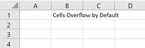
By default, when a cell contains more text than can fit in its width, the content overflows into adjacent empty cells. You can control this behavior in Spread for WPF using the AllowCellOverflow property of the GcSpreadSheet class. When AllowCellOverflow is set to false, the cell content will not overflow. The default value of this property is true.
Cell Overflow Enabled (default) | Cell Overflow Disabled |
|---|---|
|
|
Refer to the following example code to set the cell to not overflow.
C#
spreadSheet1.Workbook.ActiveSheet.Cells["B1"].Text = "Cell Does Not Overflow";
spreadSheet1.AllowCellOverflow = false;
VB
spreadSheet1.Workbook.ActiveSheet.Cells("B1").Text = "Cell Does Not Overflow"
spreadSheet1.AllowCellOverflow = False
Get and Set Cell Values
In Spread for WPF, you can get and set cell values in multiple ways. The API supports standard data types, including text, numbers, and dates.
Set Cell Values
You can assign a value to a specific cell using the IRange.Value property.
// Set cell A1 to an integer.
spreadSheet1.Workbook.ActiveSheet.Cells["A1"].Value = 12345;

// Set cell B1 to a string.
spreadSheet1.Workbook.ActiveSheet.Cells["B1"].Value = "Welcome to Spread for WPF!";

// Set cell C1 to a date.
spreadSheet1.Workbook.ActiveSheet.Cells["C1"].Value = DateTime.Today;
' Set cell A1 to an integer.
spreadSheet1.Workbook.ActiveSheet.Cells("A1").Value = 12345
' Set cell B1 to a string.
spreadSheet1.Workbook.ActiveSheet.Cells("B1").Value = "Welcome to Spread for WPF!"
' Set cell C1 to a date.
spreadSheet1.Workbook.ActiveSheet.Cells("C1").Value = DateTime.TodayAlternatively, use the SetValue method to assign a value to a cell at the specified row and column index.
// Set the value of cell (3, 3) to an integer.
spreadSheet1.Workbook.ActiveSheet.SetValue(3, 3, 10000);

// Set the value of cell (3, 4) to a string.
spreadSheet1.Workbook.ActiveSheet.SetValue(3, 4, "welcome");

// Set the value of cell (3, 5) to the current date.
spreadSheet1.Workbook.ActiveSheet.SetValue(3, 5, DateTime.Today);
' Set the value of cell (3, 3) to an integer.
spreadSheet1.Workbook.ActiveSheet.SetValue(3, 3, 10000)
' Set the value of cell (3, 4) to a string.
spreadSheet1.Workbook.ActiveSheet.SetValue(3, 4, "welcome")
' Set the value of cell (3, 5) to the current date.
spreadSheet1.Workbook.ActiveSheet.SetValue(3, 5, DateTime.Today)Get Cell Values
You can retrieve a cell's contents using either the GetValue method or the Cells[row, column].Value property. Both return an object that should be cast to the appropriate type as needed.
// Get the value of cell A1 and store it in the variable 'value'.
object value = spreadSheet1.Workbook.ActiveSheet.GetValue(0, 0);

// Get the value of cell C1 and store it in the variable 'value2'.
object value2 = spreadSheet1.Workbook.ActiveSheet.Cells[0, 2].Value;
' Get the value of cell A1 and store it in the variable "value".
Dim value As Object = spreadSheet1.Workbook.ActiveSheet.GetValue(0, 0)
' Get the value of cell C1 and store it in the variable "value2".
Dim value2 As Object = spreadSheet1.Workbook.ActiveSheet.Cells(0, 2).ValueSearch Cells
In Spread for WPF, you can use the Find method to search for specific text, numbers, or formulas within a specified cell range. The Find method provides multiple parameters such as FindLookIn, LookAt, SearchOrder, SearchDirection, etc., to enhance search functionality.
In addition, you can also use the FindNext and FindPrevious methods to find the next or previous cell that matches the same criteria.
The following code example demonstrates how to search for “0” in the “UnitsOnOrder” column, and use the FindNext method to find the next matching value within the specified cell range.
// Specify the cell range to search.
IRange f = GcSpreadSheet.Workbook.Worksheets[0].Cells["H1:H50"];

// Use the Find method to search for "0" in the range "H1:H50".
f.Find('0', null, FindLookIn.Values, LookAt.Whole, SearchOrder.Rows, SearchDirection.Next, true).Activate();

// Use the FindNext method to search for the next matching cell.
f.FindNext(GcSpreadSheet.Workbook.Worksheets[0].ActiveCell).Activate();
' Specify the cell range to search.
Dim f As IRange = GcSpreadSheet.Workbook.Worksheets(0).Cells("H1:H50")
' Use the Find method to search for "0" in the range "H1:H50".
f.Find("0"c, Nothing, FindLookIn.Values, LookAt.Whole, SearchOrder.Rows, SearchDirection.[Next], True).Activate()
' Use the FindNext method to search for the next matching cell.
f.FindNext(GcSpreadSheet.Workbook.Worksheets(0).ActiveCell).Activate()Automatic Number Formatting
In Spread for WPF, if a cell’s format is set to "General," the number format will automatically change from "General" to another format based on the current width of the cell.
Normally, when using the General format, the cell’s content is displayed exactly as entered. However, if the cell is not wide enough to display a long number in full, the value will either be rounded or shown in scientific notation (exponential form). It’s important to note that in either case, the actual value in the cell does not change—only the display format is adjusted.
For example, if you enter "72940616670583" in cell A2, as shown in the figure below, the value will be displayed as "7.29E+13" in scientific notation if the cell is not wide enough.
Create Data Types for Custom Objects
In Spread for WPF, you can set the data type of a cell to a custom object, just like in Excel.
By customizing data types, users can more conveniently extract important data from objects.
In Spread for WPF, data types are disabled by default and can be enabled by setting the CalcFeatures enumeration. For example:
GcSpreadSheet.Workbook.WorkbookSet.CalculationEngine.CalcFeatures = CalcFeatures.All;spreadSheet1.Workbook.WorkbookSet.CalculationEngine.CalcFeatures = CalcFeatures.AllThe following example code defines an Employee class with fields such as ID, First Name, Last Name, Designation, Department, Gender, Age, and Year of Joining:
[System.Reflection.DefaultMember("FirstName")]
    public class Employee
    {
        public int ID { get; set; }
        public string FirstName { get; set; }
        public string LastName { get; set; }
        public string Designation { get; set; }
        public string Department { get; set; }
        public string Gender { get; set; }
        public int Age { get; set; }
        public int YearOfJoining { get; set; }
}<System.Reflection.DefaultMember("FirstName")>
Public Class Employee
Public Property ID As Integer
Public Property FirstName As String
Public Property LastName As String
Public Property Designation As String
Public Property Department As String
Public Property Gender As String
Public Property Age As Integer
Public Property YearOfJoining As Integer
End ClassYou can use the IRichValue interface to add data types to cells, and Spread for WPF also provides a generic RichValue<T> class for wrapping any .NET object and implementing the IRichValue interface.
To add a data type to a worksheet cell, you can directly assign a custom object to the Value property of the IRange interface. When accessing object properties, you can reference them in formulas in the following ways:
Using dot notation:
B2.PropertyNameUsing square brackets:
B2.[Property Name](for property names that contain spaces)Using a function:
FIELDVALUE(B2, "PropertyName")
Note: If the property name contains spaces, you must use the square bracket syntax. For detailed information about the FIELDVALUE function, please refer to the “FIELDVALUE” entry in the function reference documentation.
The following example code demonstrates how to create a custom object, assign it to a cell, and access its properties using different syntax methods:
GrapeCity.CalcEngine.RichValue<Employee> samDaimi = new GrapeCity.CalcEngine.RichValue<Employee>(new Employee()
            {
                ID = 32700,
                FirstName = "Sam",
                LastName = "Daimi",
                Designation = "Team Lead",
                Department = "IT",
                Gender = "M",
                Age = 65,
                YearOfJoining = 2012
            });

            // Assign the object to cell B2.
            spreadSheet1.Workbook.ActiveSheet.Cells["B2"].Value = samDaimi;

            // Access properties using dot notation.
            spreadSheet1.Workbook.ActiveSheet.Cells["B3"].Formula = "B2.LastName";
            spreadSheet1.Workbook.ActiveSheet.Cells["B4"].Formula = "B2.Designation";

            // Access properties using brackets.
            spreadSheet1.Workbook.ActiveSheet.Cells["B5"].Formula = "B2.[Department]";
            spreadSheet1.Workbook.ActiveSheet.Cells["B6"].Formula = "B2.[Gender]";

            // Access properties using the FIELDVALUE function.
            spreadSheet1.Workbook.ActiveSheet.Cells["B7"].Formula = "FIELDVALUE(B2, \"Age\")";
            spreadSheet1.Workbook.ActiveSheet.Cells["B8"].Formula = "FIELDVALUE(B2, \"YearOfJoining\")";
Dim samDaimi As GrapeCity.CalcEngine.RichValue(Of Employee) = New GrapeCity.CalcEngine.RichValue(Of Employee)(New Employee() With {
.ID = 32700,
.FirstName = "Sam",
.LastName = "Daimi",
.Designation = "Team Lead",
.Department = "IT",
.Gender = "M",
.Age = 65,
.YearOfJoining = 2012
})
' Assign the object to cell B2.
spreadSheet1.Workbook.ActiveSheet.Cells("B2").Value = samDaimi
' Access properties using dot notation.
spreadSheet1.Workbook.ActiveSheet.Cells("B3").Formula = "B2.LastName"
spreadSheet1.Workbook.ActiveSheet.Cells("B4").Formula = "B2.Designation"
' Access properties using brackets.
spreadSheet1.Workbook.ActiveSheet.Cells("B5").Formula = "B2.[Department]"
spreadSheet1.Workbook.ActiveSheet.Cells("B6").Formula = "B2.[Gender]"
' Access properties using the FIELDVALUE function.
spreadSheet1.Workbook.ActiveSheet.Cells("B7").Formula = "FIELDVALUE(B2, ""Age"")"
spreadSheet1.Workbook.ActiveSheet.Cells("B8").Formula = "FIELDVALUE(B2, ""YearOfJoining"")"