Sort Data

You can sort data in a spreadsheet and specify the column or row index to sort on as well as the sort criteria. You can also specify multiple sort keys (sort by a specified column or row first, then another column or row, and so on).

Sort Range in Ascending or Descending Order

The sortRange method is used to sort data. The sortInfo object in the sortRange method specifies sort keys and ascending or descending order.

The following GIF illustrates a column sorting in ascending and descending order.

var spread = new GC.Spread.Sheets.Workbook(document.getElementById("ss"),{sheetCount:3});
var activeSheet = spread.getActiveSheet();
activeSheet.setValue(0, 0, 10);
activeSheet.setValue(1, 0, 100);
activeSheet.setValue(2, 0, 50);
activeSheet.setValue(3, 0, 40);
activeSheet.setValue(4, 0, 80);
activeSheet.setValue(5, 0, 1);
activeSheet.setValue(6, 0, 65);
activeSheet.setValue(7, 0, 20);
activeSheet.setValue(8, 0, 30);
activeSheet.setValue(9, 0, 35);

$("#button1").click(function(){
     //Sort Column1 by ascending at every button click.
    activeSheet.sortRange(-1, 0, -1, 1, true, [{index:0, ascending:true}]);
   });
 $("#button2").click(function(){
    //Sort Column1 by descending at every button click.
     activeSheet.sortRange(-1, 0, -1, 1, true, [
       {index:0, ascending:false}
     ]);
 });
//Add button controls to the page

Sort Multiple Ranges

You can sort multiple ranges by specifying multiple sort keys in the sortInfo object.

$(document).ready(function ()
{
    var spread =
    new GC.Spread.Sheets.Workbook(document.getElementById("ss"), {sheetCount:3});
    var activeSheet = spread.getActiveSheet();
    activeSheet.setRowCount(6);
    activeSheet.setValue(0, 0, 10);
    activeSheet.setValue(1, 0, 100);
    activeSheet.setValue(2, 0, 100);
    activeSheet.setValue(3, 0, 10);
    activeSheet.setValue(4, 0, 5);
    activeSheet.setValue(5, 0, 10);
    activeSheet.setValue(0, 1, 10);
    activeSheet.setValue(1, 1, 40);
    activeSheet.setValue(2, 1, 10);
    activeSheet.setValue(3, 1, 20);
    activeSheet.setValue(4, 1, 10);
    activeSheet.setValue(5, 1, 40);
    $("#button1").click(function()
    {
        // Create a SortInfo object where 1st Key:Column1 / 2nd Key:Column2.
        var sortInfo =
        [
            {index:0, ascending:true},
            {index:1, ascending:false}
        ];
        // Execute sorting which targets all rows based on the sorting conditions.
        spread.getActiveSheet().sortRange(0, 0, 6, 2, true, sortInfo);
    });
});

//Add button control to page

Sort by Cell Background Color

You can sort the cells by background color using the sortInfo.backColor option. The cells are grouped by position at the top or bottom of the selected range using the sortInfo.order option.

The following GIF illustrates the green-colored cells being sorted at the bottom.

sheet.setArray(0, 0, [
    ["Order No.","Order Date","Product Type","Qty","Customer ID","Delivery Status"],
    ["1234", "11-Jul", "Electronic", "1", "861861", "Delivered"],
    ["1235", "12-Jul", "Clothing",   "4", "530317", "Past Due"],
    ["1236", "13-Jul", "Cleaning",   "2", "753904", "Past Due"],
    ["1237", "14-Jul", "Food Item",  "6", "623424", "Delivered"],
    ["1238", "15-Jul", "Electronic", "3", "214403", "Past Due"],
    ["1239", "16-Jul", "Clothing",   "7", "105146", "Due in 4 Days"],
    ["1240", "17-Jul", "Cleaning",   "3", "860876", "Past Due"],
    ["1241", "18-Jul", "Food Item",  "8", "126990", "Delivered"],
    ["1242", "19-Jul", "Electronic", "2", "505788", "Delivered"],
    ["1243", "20-Jul", "Clothing",   "5", "298332", "Due in 4 Days"]
]);
            
spread.getSheet(0).getCell(1, 5).backColor("#E2EFDA");            
spread.getSheet(0).getCell(2, 5).backColor("#FCE4D6");            
spread.getSheet(0).getCell(3, 5).backColor("#FCE4D6");            
spread.getSheet(0).getCell(4, 5).backColor("#E2EFDA");            
spread.getSheet(0).getCell(5, 5).backColor("#FCE4D6");            
spread.getSheet(0).getCell(6, 5).backColor("#FFF2CC");            
spread.getSheet(0).getCell(7, 5).backColor("#FCE4D6");            
spread.getSheet(0).getCell(8, 5).backColor("#E2EFDA");            
spread.getSheet(0).getCell(9, 5).backColor("#E2EFDA");            
spread.getSheet(0).getCell(10, 5).backColor("#FFF2CC");

var ColorList = new GC.Spread.Sheets.CellTypes.RadioButtonList();
ColorList.items([
    { text: "Green", value: "green" },
    { text: "Red", value: "red" }, 
    { text: "Yellow", value: "yellow" }
]);
spread.getSheet(0).getCell(12, 2).cellType(ColorList);

var OrderList = new GC.Spread.Sheets.CellTypes.RadioButtonList();
OrderList.items([
    { text: "Top", value: "top" },
    { text: "Bottom", value: "bottom" }
]);
spread.getSheet(0).getCell(12, 3).cellType(OrderList);
  
sortBackColor(spread.getSheet(0));
    
function sortBackColor (sheet){
    const CELL_COLOR_MAPPING = {
        green: "#E2EFDA",
        red: "#FCE4D6",
        yellow: "#FFF2CC",
    }
    sheet.setColumnWidth(3,120);
    var style = new GC.Spread.Sheets.Style();
    style.cellButtons = [{
    caption: "Sort By Cell Color",
    useButtonStyle:true,
    width: 120,
    command: function (sheet) {
        var value = sheet.getValue(12,2);
        var order = sheet.getValue(12,3);
        value = value ? value : "green";
        order = order ? order : "top";
        var color = CELL_COLOR_MAPPING[value];
        sheet.sortRange(1,0,10,6,true,[{
            index:5,
            backColor:color,
            order:order,
        }])
    }
    }];
    sheet.setStyle(13,3,style);
}

Using SpreadJS Designer

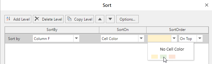
You can sort by background color by choosing the "Cell Color" option in the "SortOn" dropdown. The Sort dialog can be accessed from Home > Editing > Sort & Filter > "Custom Sort" option.

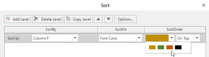
Sort by Font Color

You can sort the cells by font color using the sortInfo.foreColor option. The cells are grouped by position at the top or bottom of the selected range using the sortInfo.order option.

The following GIF illustrates red-colored cells being sorted at the top.

spread.getSheet(1).setArray(0, 0, [
    ["Order No.","Order Date","Product Type","Qty","Customer ID","Delivery Status"],
    ["1234", "11-Jul", "Electronic", "1", "861861", "Delivered"],
    ["1235", "12-Jul", "Clothing",   "4", "530317", "Past Due"],
    ["1236", "13-Jul", "Cleaning",   "2", "753904", "Past Due"],
    ["1237", "14-Jul", "Food Item",  "6", "623424", "Delivered"],
    ["1238", "15-Jul", "Electronic", "3", "214403", "Past Due"],
    ["1239", "16-Jul", "Clothing",   "7", "105146", "Due in 4 Days"],
    ["1240", "17-Jul", "Cleaning",   "3", "860876", "Past Due"],
    ["1241", "18-Jul", "Food Item",  "8", "126990", "Delivered"],
    ["1242", "19-Jul", "Electronic", "2", "505788", "Delivered"],
    ["1243", "20-Jul", "Clothing",   "5", "298332", "Due in 4 Days"]
]);

spread.getSheet(1).name("Sort by font color");
spread.getSheet(1).getCell(1, 5).foreColor("#548235");            
spread.getSheet(1).getCell(2, 5).foreColor("#C65911");            
spread.getSheet(1).getCell(3, 5).foreColor("#C65911");            
spread.getSheet(1).getCell(4, 5).foreColor("#548235");            
spread.getSheet(1).getCell(5, 5).foreColor("#C65911");            
spread.getSheet(1).getCell(6, 5).foreColor("#BF8F00");            
spread.getSheet(1).getCell(7, 5).foreColor("#C65911");            
spread.getSheet(1).getCell(8, 5).foreColor("#548235");            
spread.getSheet(1).getCell(9, 5).foreColor("#548235");            
spread.getSheet(1).getCell(10, 5).foreColor("#BF8F00");

var FontColorList = new GC.Spread.Sheets.CellTypes.RadioButtonList();
FontColorList.items([
    { text: "Green", value: "green" },
    { text: "Red", value: "red" }, 
    { text: "Yellow", value: "yellow" }
]);
spread.getSheet(1).getCell(12, 2).cellType(FontColorList);

var FontColorOrder = new GC.Spread.Sheets.CellTypes.RadioButtonList();
FontColorOrder.items([
    { text: "Top", value: "top" },
    { text: "Bottom", value: "bottom" }
]);
spread.getSheet(1).getCell(12, 3).cellType(FontColorOrder);
  
sortFontColor(spread.getSheet(1));

function sortFontColor (sheet){
    const FONT_COLOR_MAPPING = {
        green:"#548235",
        red:"#C65911",
        yellow: "#BF8F00"
    }
    sheet.setColumnWidth(3,120);
    var style = new GC.Spread.Sheets.Style();
    style.cellButtons = [{
            caption:"Sort By Font Color",
            useButtonStyle:true,
            width:120,
            command:function (sheet){
                var value = sheet.getValue(12,2);
                var order = sheet.getValue(12,3);
                value = value ? value : "green";
                order = order ? order : "top";
                var color = FONT_COLOR_MAPPING[value];
                sheet.sortRange(1,0,10,6,true,[{
                    index:5,
                    fontColor:color,
                    order:order
                }])
            }
        }];
    sheet.setStyle(13,3,style);
}

Using SpreadJS Designer

You can sort by font color by choosing the "Font Color" option in the "SortOn" dropdown. The Sort dialog can be accessed from Home > Editing > Sort & Filter > "Custom Sort" option.

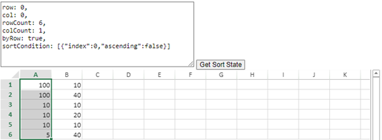
Keep the Last Sort State

You can preserve the default or last-applied state of data before you sort it, which does not change whenever a different sort order is applied. You can use the getSortState method to get the current worksheet’s last sort state whenever required and for reordering the range of data, the sortRange method can be used.

Refer to the following image that depicts a preserved sort state.

lastsortstate

The following code sample implements the sheet’s ValueChanged event which calls the getSortRange method to restore the sorted state and then uses the sortRange method whenever any change is detected in the sorting area.

// To call automatic sorting every time any value is changed.
sheet.bind(GC.Spread.Sheets.Events.ValueChanged, function (e, info) {
     let sortState = sheet.getSortState();
     if (inSortStateRange(sortState, info.row, info.col)) {
         sheet.sortRange();
     }
});

Note:
This feature supports export/import for SSJSON, SJS, and XLSX.
Filtering with worksheet.getsortState() does not return the sort state.

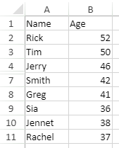
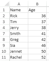
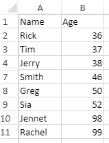
Ignore Hidden Data while Sorting

You can also skip hidden data while sorting by using the ignoreHidden option in API. A cell or a range is considered to be hidden when:

A row's height or column's width is 0
A row or column is hidden
A row or column is filtered out
Some rows or columns are grouped and unexpanded

The below example contains hidden rows (cells A5:A6) and displays how the data is sorted with different values of ignoreHidden :

Original Data	ignoreHidden is true	ignoreHidden is false

The following code sample shows how to sort data by skipping hidden rows.

// get the activesheet
var activeSheet = spread.getSheet(0);
// Set data
activeSheet.setValue(0, 0, "Name");
activeSheet.setValue(0, 1, "Age");
activeSheet.setValue(1, 0, "Rick");
activeSheet.setValue(1, 1, 52);
activeSheet.setValue(2, 0, "Tim");
activeSheet.setValue(2, 1, 50);
activeSheet.setValue(3, 0, "Jerry");
activeSheet.setValue(3, 1, 46);
activeSheet.setValue(4, 0, "Jack");
activeSheet.setValue(4, 1, 98);
activeSheet.setValue(5, 0, "Sandy");
activeSheet.setValue(5, 1, 99);
activeSheet.setValue(6, 0, "Smith");
activeSheet.setValue(6, 1, 42);
activeSheet.setValue(7, 0, "Greg");
activeSheet.setValue(7, 1, 41);
activeSheet.setValue(8, 0, "Sia");
activeSheet.setValue(8, 1, 36);
activeSheet.setValue(9, 0, "Jennet");
activeSheet.setValue(9, 1, 38);
activeSheet.setValue(10, 0, "Rachel");
activeSheet.setValue(10, 1, 37);
// Hide Row
activeSheet.setRowHeight(4, 0.0, GC.Spread.Sheets.SheetArea.viewport);
activeSheet.setRowHeight(5, 0.0, GC.Spread.Sheets.SheetArea.viewport);

// Sort range i.e. "Age" column with ignoreHidden set to true
activeSheet.sortRange(1, 1, 10, 1, true, [{ index: 1, ascending: true }], { ignoreHidden: true });

SpreadJS also allows you to sort grouped data by using groupSort enumeration. The grouped and unexpanded data is considered as hidden rows or columns. To know more about sorting grouped data, refer to Sort with Grouped Data.

The behavior of data when groupSort and ignoreHidden are used together, is explained in the below table:

	ignoreHidden=true	ignoreHidden=false	ignoreHidden undefined
groupSort (group, child or full)	Group sort works, and hidden values are not ignored
groupSort (flat)	Ignores hidden values	Does not ignore hidden values	Ignores hidden values
groupSort undefined	Ignores hidden values	Does not ignore hidden values	If the sorting range contains a group, then group sort is applied. If the sorting range does not contain a group, then hidden values are ignored

ignoreHidden=true

ignoreHidden=false

ignoreHidden undefined

groupSort (group, child or full)

Group sort works, and hidden values are not ignored

groupSort (flat)

Ignores hidden values

Does not ignore hidden values

Ignores hidden values

groupSort undefined

Ignores hidden values

Does not ignore hidden values

If the sorting range contains a group, then group sort is applied.

If the sorting range does not contain a group, then hidden values are ignored

The following code sample shows how to use ignoreHidden and groupSort together.

// set data
 activeSheet.setArray(3, 0, [
     [6221], [5125], ['Samsung'], [4348], [3432], ['LG'], [1928], [2290], ['Oppo'], [8939], [7006], ['Apple']
 ]);
 activeSheet.rowOutlines.group(3, 2);
 activeSheet.rowOutlines.group(6, 2);
 activeSheet.rowOutlines.group(9, 2);
 activeSheet.rowOutlines.group(12, 2);
 spread.resumePaint();

 // set rowFilter
 activeSheet.rowFilter(new GC.Spread.Sheets.Filter.HideRowFilter(new GC.Spread.Sheets.Range(3, 0, 13, 1)));

 // hide rows
 activeSheet.setRowHeight(4, 0.0, GC.Spread.Sheets.SheetArea.viewport);
 activeSheet.setRowHeight(5, 0.0, GC.Spread.Sheets.SheetArea.viewport);

 //1) If you want to use filter dialog to sort the data with enhanced group feature and ignoreHidden, you should use RangeSorting event
 spread.bind(GC.Spread.Sheets.Events.RangeSorting, function (e, info) {
     // set GroupSort to full
     info.groupSort = GC.Spread.Sheets.GroupSort.full;
     // set ignoreHidden to true
     info.ignoreHidden = true;
 });

 //2) If you want to use api to sort the data with enhanced group feature and ignoreHidden, you should use this code
 // activeSheet.sortRange(3, 0, 13, 1, true, [{ index: 0, ascending: true }], { ignoreHidden: true, groupSort: GC.Spread.Sheets.GroupSort.full });

Exclude Data Headers when Sorting

When sorting data in a worksheet, users often need to keep the header row fixed so that column titles are not sorted along with the data.

SpreadJS automatically detects header rows in the selected range and can exclude them from the sort.

Feature Availability

Accessible in the Custom Sort dialog within the SpreadJS Designer.
Works with tables, normal ranges, and filtered datasets (with conditions).
Header detection applies only to top-to-bottom sorting.

Key Benefits

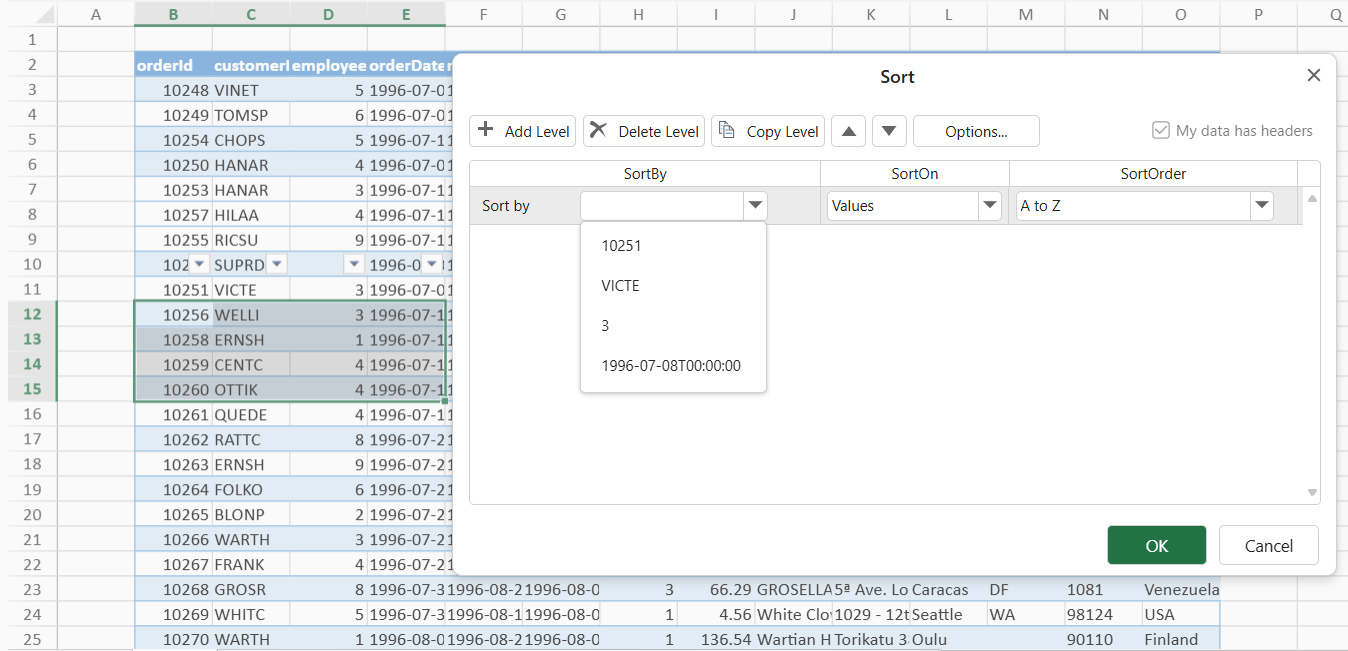
Automatic Header Detection
SpreadJS automatically detects and separates the header row from the data range.
The detection primarily evaluates the top row of the selected range and, if needed, the row immediately above it.
The evaluation is based on differences in cell type, content, or style between the first two rows (partial blanks are allowed).
If no clear header can be identified, the first row of the current selection is used as the header by default.
Simplified Workflow
Users can sort entire datasets directly — headers are preserved automatically, reducing the chance of mis-sorted column titles.
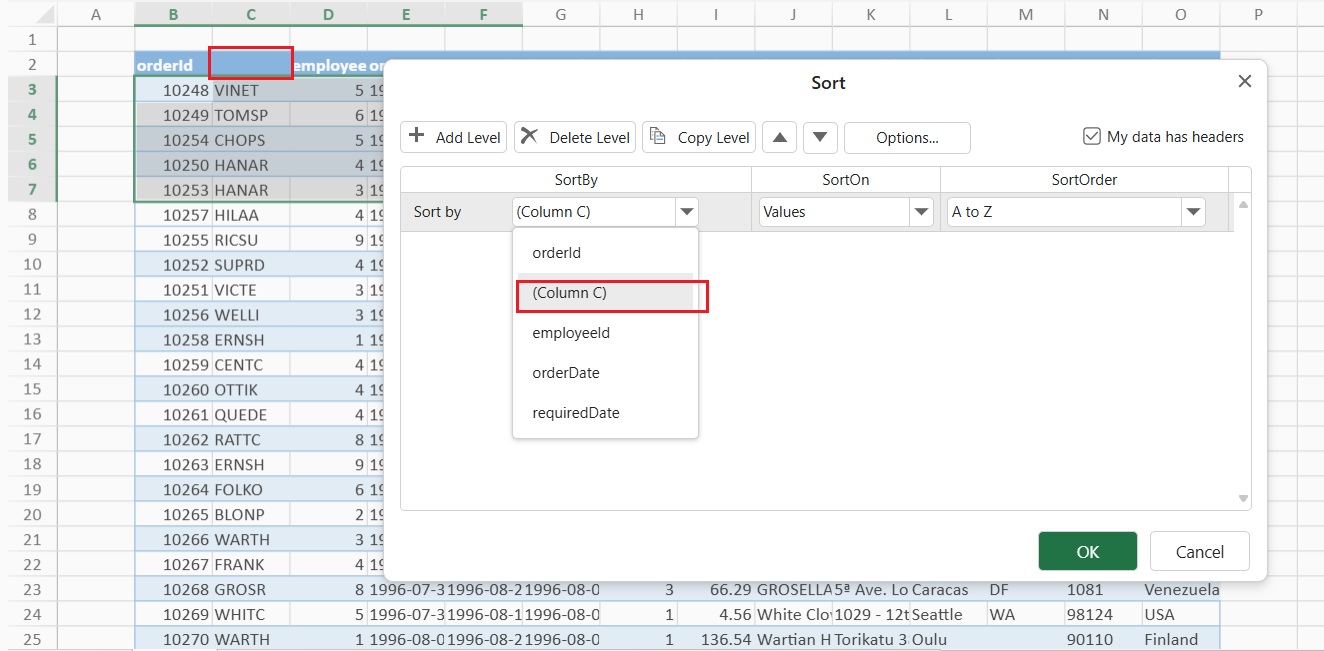
Accurate Sorting Labels
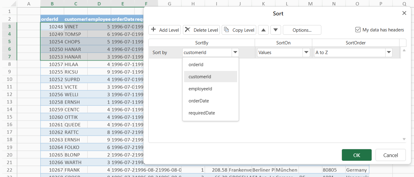
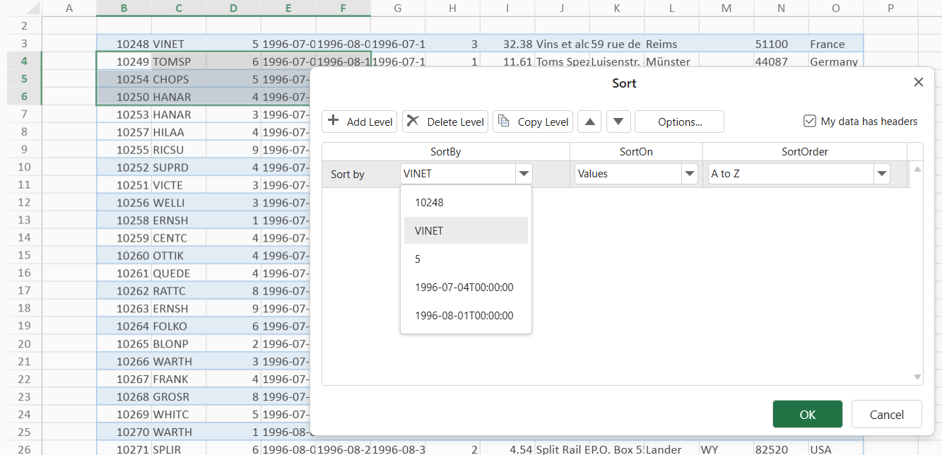
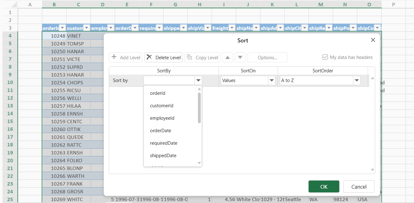
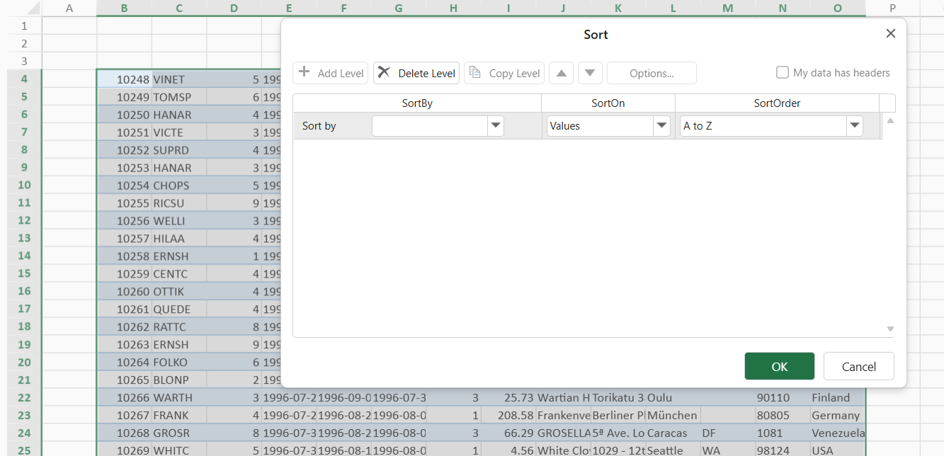
When headers are detected, the column names shown in the Sort dialog reflect the text in the header cells.
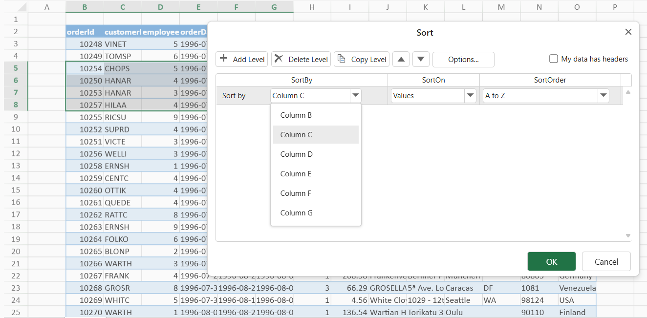
If the “My Data Has Headers” option is cleared, the Sort dialog displays column letters (for example, Column A, Column B) instead of header text.

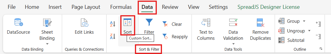
Operations

Step 1: Select the range of data in the worksheet that you want to sort.

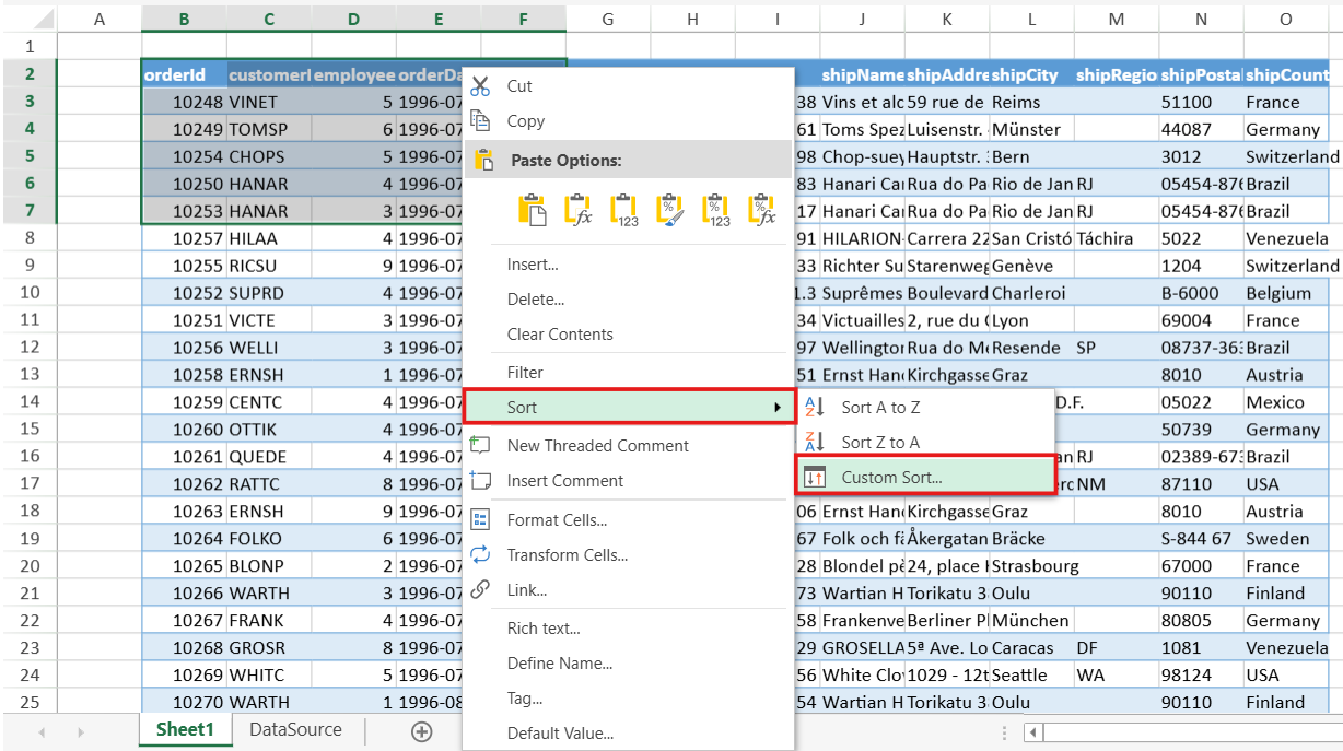
Step 2: Open the Custom Sort dialog by using one of the following methods:

Method 1: On the Data tab, in the Sort & Filter group, click Sort.
Method 2: Right-click the selected range, point to Sort, and then select Custom Sort from the context menu.

Sorting Behavior

Scenario	Behavior	Examples
Range with Recognizable Headers	“My Data Has Headers” box is automatically selected. The SortBy list in the Sort dialog displays header text.	Range with Headers: Range without Headers:
Range Without Recognizable Headers	“My Data Has Headers” box is cleared. The SortBy list in the Sort dialog displays a default column reference (for example, Column A, Column B) in the Sort dropdown.
Table with Headers Shown	“My Data Has Headers” is selected and unavailable. Sorting applies to all rows. SpreadJS automatically manages header exclusion.
Table with Headers Hidden	The “My Data Has Headers” option is cleared and unavailable. Sorting applies to all rows. The SortBy list in the Sort dialog displays a default column reference (for example, Column A, Column B).
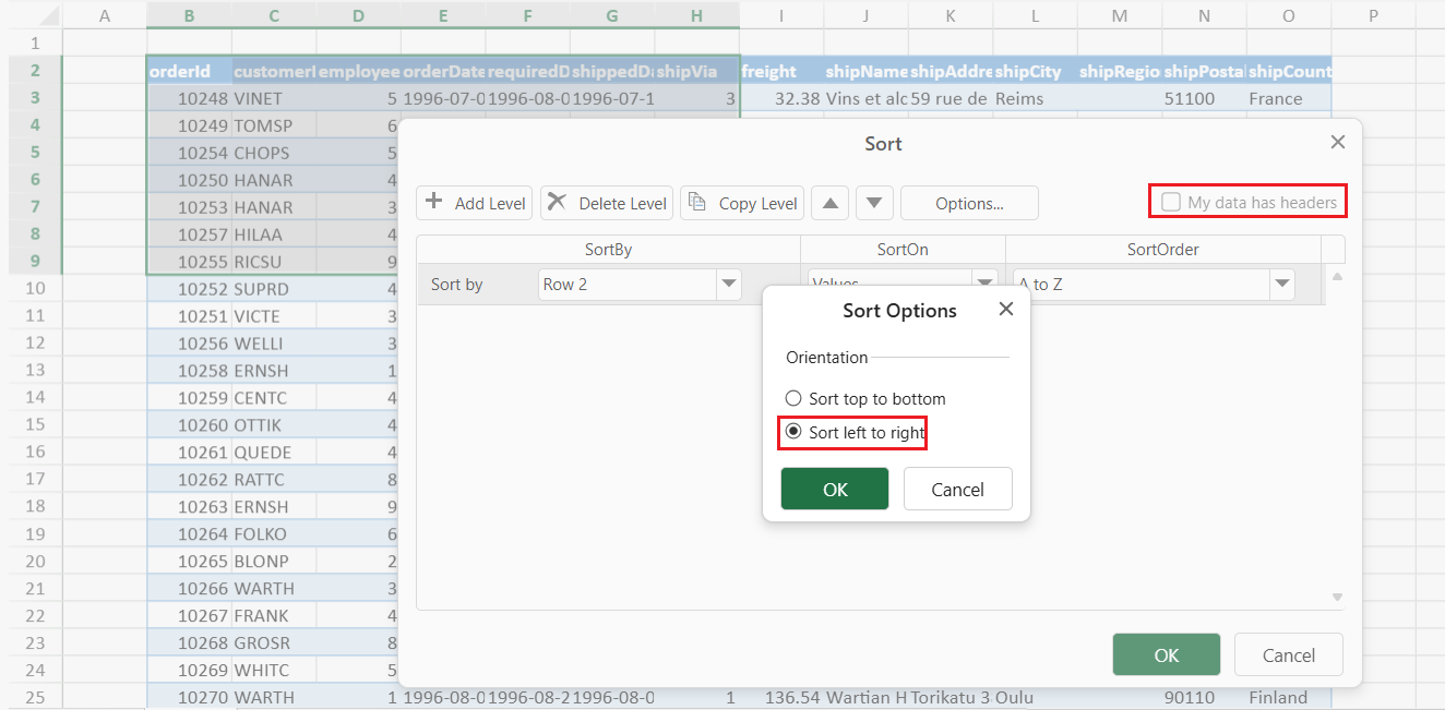
Filtered Range	The "My Data Has Headers" option is unavailable.
Left-to-Right Sort Orientation	The "My Data Has Headers" option is unavailable.
The Header Row Contains Empty Cells	The SortBy list in the Sort dialog displays a default column reference (for example, Column A, Column B).

Notes:
Custom Sort memory: The Custom Sort dialog automatically remembers your last sorting configuration for each selected range. You can reopen it later to review or adjust the existing sort levels and order.
One‑click Sort behavior: When you use the one‑click Sort A→Z or Sort Z→A commands:
If no custom sort has been performed since the file was opened, SpreadJS automatically checks whether the first row in the current selection is a header row and excludes it from sorting.
After a custom sort has been executed, the last state of the “My data has headers” option is remembered and applied to all subsequent one‑click sorts in the same session.