Retrieve Pivot Table Ranges and Data

DsExcel allows you to retrieve specific ranges and data from your pivot table.

• Retrieve Pivot Table Ranges

• Get Pivot Table Data

Retrieve Pivot Table Ranges

The structure of a pivot table report is comprised of different ranges. In order to retrieve a specific range of pivot table, it is important to understand the structure of a pivot table.

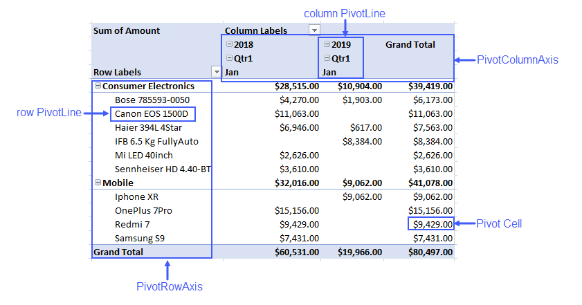
As can be observed from the above screenshot, the structure of a pivot table can be explained as:

• PivotRowAxis: The row axis area of a pivot table contains fields which group the table's data by rows

• PivotColumnAxis: The column axis area of a pivot table contains fields which break the table's data into different categories by columns.

• Pivot Cell: Any cell in a pivot table

• Row PivotLine: Any row in the row axis area of a pivot table

• Column PivotLine: Any column in the column axis area of a pivot table

DsExcel provides API to retrieve the detailed ranges of a pivot table to apply any operation or style on them to make the result more readable and distinguishable. Detailed pivot table ranges which can be retrieved are:

• Different types of pivot cells like subtotals, grand totals, data fields, pivot fields, values, blank cells

• Different types of pivot lines like subtotal, grand total, regular or blank line

• Entire row or column axis

• Whole page area

• Entire pivot table report including page fields

• A value in any range of pivot table

• The position of any element or pivot line

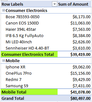
Refer to the following example code to get a specific range and set its style in a pivot table report.

//get detail range and set style
foreach (var item in pivottable.PivotRowAxis.PivotLines)
{
    if (item.LineType == PivotLineType.Subtotal)
    {
        item.PivotLineCells[0].Range.Interior.Color = Color.GreenYellow;
    }
}

The output of above code example when viewed in Excel, looks like below

Get Pivot Table Data

DsExcel.NET provides GETPIVOTDATA function which queries the pivot table to fetch data as per the specified parameters. The main advantage of using this function is that it ensures that the correct data is returned, even if the pivot table layout has changed.

Syntax

=GETPIVOTDATA(data_field, pivot_table, [field1, item1, field2, item2],…)

GETPIVOTDATA function can be implemented to return a single cell value or a dynamic array depending on the parameters we are passing. To retrieve a single cell value, name of the data field and pivot table are mandatory parameters. While the third parameter which is a combination of field names and item names, is optional. However, for retrieving a dynamic array, all three parameters are required and the item name supports array like {“Canada”, “US”, “France”) or a range reference like A1:A3. Also, you must use IRange.Formula2{get;set;} for GETPIVOTDATA function to return a dynamic array which is spilled across a range. For ease of use, you can also automatically generate GETPIVOTDATA function by using the IRange.GenerateGetPivotDataFunction method. However, the GenerateGetPivotDataFunction method returns null when the IRange object is not a single cell.

Refer to the following example code for GETPIVOTDATA function returning a single cell:

// GenerateGetPivotDataFunction method is used to generate formula automatically for the selected cell
var worksheet2 = workbook.Worksheets.Add();
worksheet.Range["H25"].Formula = worksheet.Range["G6"].GenerateGetPivotDataFunction(worksheet2.Range["A1"]);

// Here, the GETPIVOTDATA function is used to fetch the desired result
worksheet2.Range["H24"].Formula = @"=GETPIVOTDATA(""Amount"",Sheet1!$A$1,""Category"",""Mobile"",""Country"",""Australia"")";

Refer to the following example code for GETPIVOTDATA function returning a dynamic array:

// Here, Formula2 is used along with GETPIVOTDATA to fetch the multiple values
worksheet.Range["H10"].Formula2 = @"=GETPIVOTDATA(""Amount"",$A$1,""Category"",""Consumer Electronics"",""Country"",{""Canada"",""Germany"",""France""})";